MIRR Function in Excel – Modified Internal Rate of Return

MIRR Function in Excel is a modified form of IRR. IRR considers that the money reinvests at the same discount rate. In finance, most of the time we have a different borrowing rate and reinvestment rate. MIRR covers that limitation of IRR.

Here we go 😎

When to Use MIRR Function of Excel

The word MIRR represents “Modified Internal Rate of Return”. In a project, MIRR accounts for two factors i.e borrowing rate and reinvestment rate. Generally, the reinvestment rate is lower than the borrowing rate. We use the MIRR when the interest money is reinvested at a different rate from the rate at which invested amount was borrowed.

The MIRR Function comes under the category of Financial functions of Excel.

Syntax and Arguments

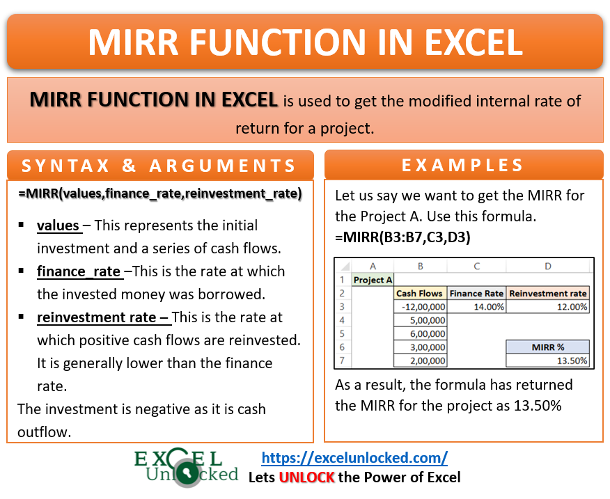
=MIRR(values,finance_rate,reinvestment_rate)

The following points contain the required information regarding MIRR function arguments.

• values – values represent the initial investment and a series of cash flows after the investment.
• finance_rate – This is the rate at which a company borrows the invested money. The rate is for negative cash flows as well.
• reinvestment_rate – This is the rate at which a company reinvests the positive cash flows.

Points to Know about MIRR Function of Excel

The following points should be kept in mind before using the MIRR function in Excel.

• The values function argument works in a chronological way. It assumes that there is a time interval of one year between each cash flow.
• The function considers that all the cash inflows and outflows occur at the end of period.
• We can use MIRR Function to compare two projects that have same NPV. Any company will go for the project with more MIRR.
• The finance_rate is zero when the company has its own money to invest and it does not account for any borrowing rate.
• values function argument must contain at least one negative and one positive value.

Examples for MIRR Function in Excel

In this section of the blog, we have taken some practical examples with result verification for each to learn the MIRR function usage.

Ex.1 – Simplest Example for MIRR Function in Excel

Let us assume that a company is deciding to invest the money in building a new Airport. The following are the cash flows for this project.

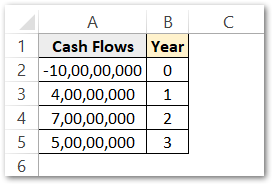
The initial investment is negative as it is a cash outflow.

The invested money is at a zero finance rate. While the positive cash flows are reinvested at a rate of 6%. Use the following MIRR formula.

=MIRR(A2:A5,0,6%)

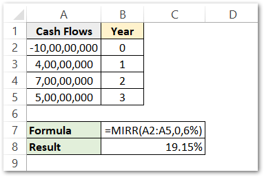
As a result, the formula has returned the MIRR as 19.15%.

Explanation – We have passed the range A2:A5 as the values function argument. The finance rate is zero while the reinvestment rate is 6% ( or 0.6 ). Both the finance rate and reinvestment rate are directly written into the formula instead of using the cell references. As a result, the formula has returned the MIRR of this project to be 19.15 percent.

Ex.1 Result Verification

As we know, while working with finances some smart workers have a habit to double-check everything they calculated using predefined functions.

Below is the formula used to get the Future Value Factor for the future cash flows at a 6% reinvestment rate.

=(1+0.06)^(3-B3)

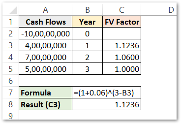
We have used the excel fill handle tool to copy the formula to cells C4 and C5.

Explanation – We have used the formula to get the FV factor. The FV factor is the percentage we used to get the terminal or future values of cash inflows after being reinvested. Look at cell A3 containing the cash inflow for the first year. This amount of 4 crores is reinvested at 6% or 0.06 interest till the end of this project, The money is invested at the end of the first year to the end of the third year ( end of the project ) which makes the number of years as 3-B3 i.e 2. This FV factor when multiplies with cash flow, gives us the money we will receive at the end of the project as the inflow is compounded annually till the end of the project.

After that, we will calculate the terminal value for the positive cash flows ( A3, A4, A5 )

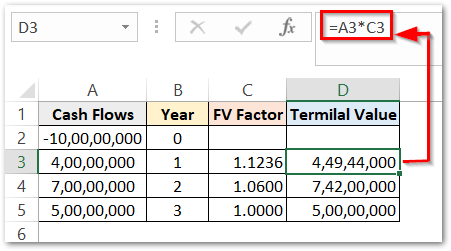
Now use this formula to get the MIRR percentage.

=POWER(SUM(D3:D6)/-A2,1/B5)-1

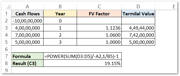
As a result, the formula has returned MIRR % as 19.15%. We have got the same result when we used the MIRR function in the 1st example. Hence it verifies the result.

Explanation – The general formula to get MIRR is

MIRR = (PVCO/FVCI)^1/n -1

PVCO= Present value of cash outflows (A2)

FVCI = Future value of cash inflows ( Sum of D3, D4, D5 )

n = number of total years ($B$5)

Thus this formula returns the MIRR manually.

Ex.2 – Comparing the Projects using MIRR Function

Let us say there are two Projects A and B. The project cash flows, finance rate, and reinvestment rates are given below.

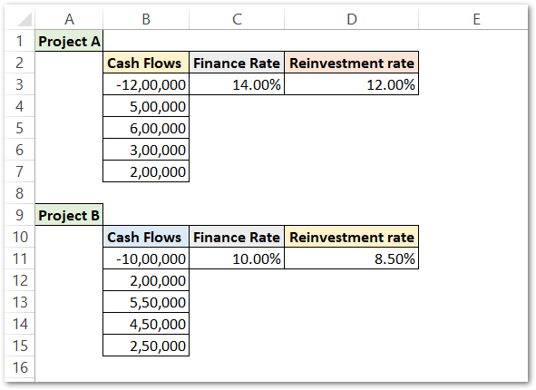
Use the following formulas in cells D7 and D15 to get MIRR (using MIRR function in Excel) for projects A and B respectively.

=MIRR(B3:B7,C3,D3)

=MIRR(B11:B15,C11,D11) 

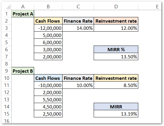
As a result, the formula has returned MIRR for projects A and B as 13.50 % and 13.19 %. Project A has more MIRR, so it will be preferred first to invest money in.

Explanation – The values function argument has the range B3:B7 that contains the cash flows for project A. Finance rate and reinvestment rates are C3 and D3 respectively. So the MIRR function returns the modified internal rate for project A.

The formula works in the same way for Project B.

Note that the initial investments are negative for both the projects in cells B3 and B11 otherwise, the formula will return a #DIV!0 error.

Thank you for reading 😉