ISPMT Function of Excel – Interest Amount Keeping the Principal Constant

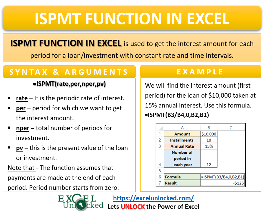
In our earlier blogs, we learned the usage of the IPMT Function to get the interest amount when the payment ( principal+interest ) was constant for each period. The ISPMT Function in Excel also gives us interest amounts for a specific period but with a different concept.

Here we go 😎

When to Use ISPMT Function of Excel

The ISPMT Function in Excel comes into its use when we want to get the interest amount for any period during an investment. The function first divides the initial value of the investment by the total number of periods to get the constant periodic principal amount.

The ISPMT Function can be categorized under the Financial Functions of Excel.

Syntax and Argument

=ISPMT(rate,nper,per,pv)

The below points contain the information about Excel ISPMT Function.

• rate – This is the percentage for interest to be paid with the principal amount in each period.
• per – This is the period for which we want to get the interest amount.
• nper – The argument represents the total number of periods.
• pv – This is the initial amount or present value. It is the loan amount in case of a loan.

Points to Remember About ISPMT Function in Excel

One should always keep the following points about ISPMT Function in mind to have its successful running.

• With a constant periodic principal, it means that if the total loan amount is 10,000. We need to pay 2,000 for each period as principal ( interest with it ) for five periods.
• The payment amount is never constant in this case. This is why because payment = principal + interest, where interest for each period is not constant.
• The period number starts from 0 and not 1. First period will lead to an input parameter of nper as 0. Similary, we need to use 1 for the 2nd period.
• The function assumes that payments are being done at the end of period.
• The cash inflow is positive while the cash outflow is negative.
• We need to convert the rate percentage if, the annual rate is (let it be 10%), monthly (10%/12) , quarterly (10%/4) or semi-annually (10%/2).
• per should be an integer between 0 and nper-1.

Examples to Learn ISPMT Function in Excel

In this section of the blog, we will learn some practical examples to learn the usage of ISPMT Function in excel

Ex.1 – Simplest Example for ISPMT Function in Excel

In this example let us say a person borrowed $10,000 on 15% annual interest. The person has promised to pay back the amount in 10 equal installments. Below is the data.

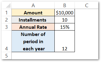
Use the following formula of excel to get the interest amount for the first period.

=ISPMT(B3/B4,0,B2,B1)

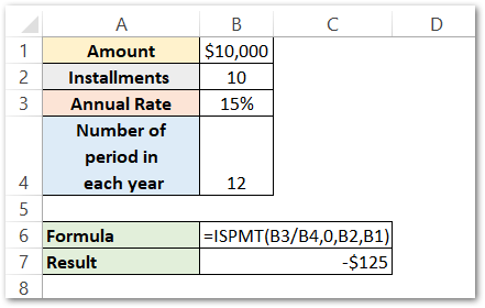
As a result, the function has returned -$125.

Explanation – This has to be explained via ISPMT Function arguments.

• rate – The annual rate in cell B3 is converted to periodic rate by dividing the annual rate (B3) by the number of periods in each year (B4). So the periodic rate becomes B3/B4.
• per – per is 0 because we want to get the interest amount for the first period.
• nper – there is a total number of 10 (B2) installments for this money to be returned back.
• pv – pv is the present value of the loan amount (B1).

The function returns a negative $125 because the interest amount for the first period debits from the borrower’s account.

Similarly, we can get the amount of interest amount for each period. Use this formula.

=ISPMT($B$3/$B$4,D2-1,$B$2,$B$1)

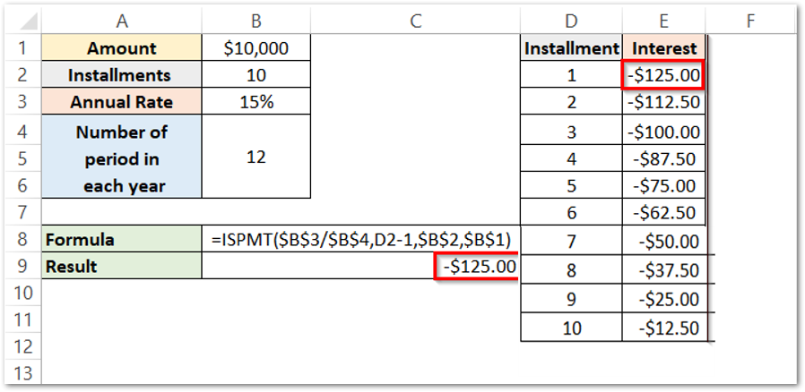
As a result, the ISPMT Function returns the interest amount for each installment of the loan. We have subtracted 1 from the installment number to get the per (D2-1). The formula is copied using the excel fill handle tool.

Note that, =ISPMT($B$3/$B$4,D2-1,$B$2,$B$1) in this formula we have used absolute and relative cell referencing. rate, nper, and pv are in absolute reference ($) to keep the cell reference locked while the per is in relative referencing so that when we copy the formula, the per changes as per the installment number.

Ex.2 – Getting the Quarter-wise Interest Amount for a Loan

Let us say, this time the person took a loan of $150,000 from the bank quarterly. The annual rate of interest is 10%. The payments clear one after another at the end of each quarter.

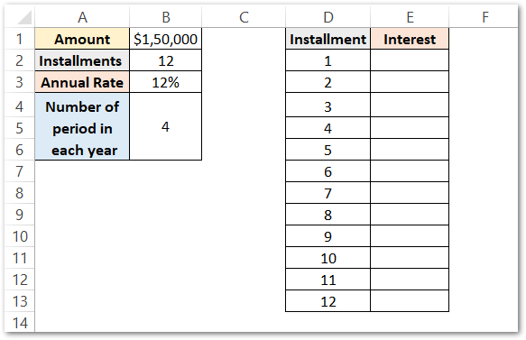
There is a total of 12 installments for the loan to get paid off. Each installment pays at the end of three months ( a quarter ). It will take a total of 12 quarters or 3 years to completely settle the loan. Use this formula to get the amount of interest for each period ( 1 to 12 quarters ).

=ISPMT($B$3/$B$4,D2-1,$B$2,$B$1)

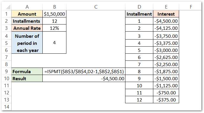
As a result, the formula has returned the interest amount for the 1st period (E2). We have copied the formula down for the rest of the installments in column E.

Explanation – Check the required function arguments used in this case.

• rate – The annual rate in cell B3 converts to periodic rate by dividing the annual rate (B3) by the number of periods in each year (B2). So the periodic rate becomes B3/B4.
• per – per is always one less than the actual number of periods. 1 is subtracted from the installments (D2). It becomes D2-1
• nper – there is a total number of 12 (B2) quarters for this money to return.
• pv – pv is the present value of the loan amount (B1).

Also, keep in mind that we have used absolute referencing for rate, nper, and pv so that their cell references do not shift down when we copy the formula. There is relative referencing for per.

Thank you for reading 😉

Frequently Asked Questions