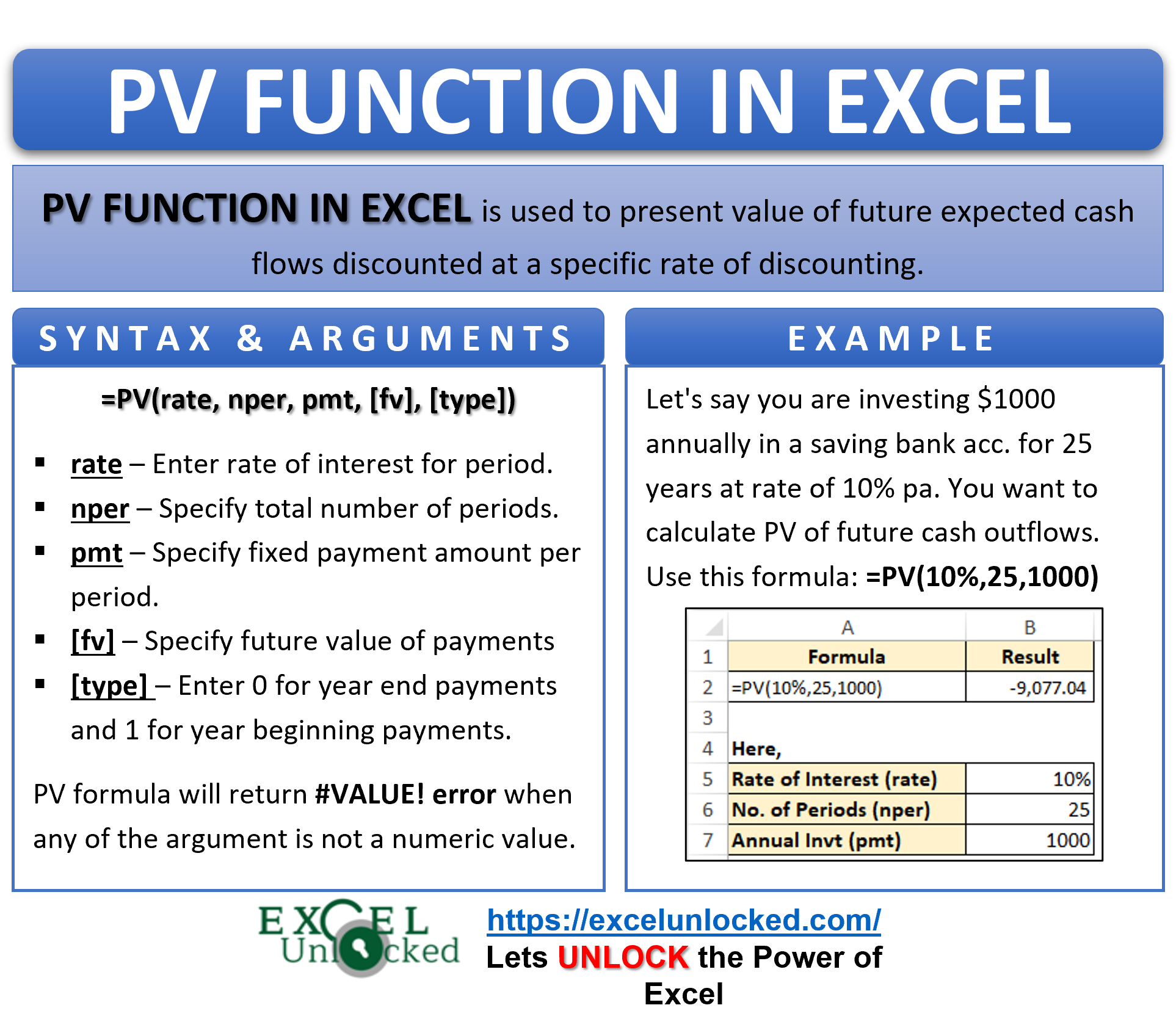
The term PV represents Present Value. In this tutorial, we would learn about an excel formula function to calculate the present value (PV) of future cash flows. The cash flows may be from an investment, or loan, or insurance, etc.
In this blog, we would learn how to use the PV function in excel to find the present value of an investment or any other cash-flow generating option.
When To Use Excel PV Function
PV formula is an Excel financial function which returns the present value of future cash flows from an investment based on the specific interest rate.
This function is useful to find the dollar present value for both – multiple periodic cash flows and also single lump-sum payments.
Syntax and Arguments
=PV(rate, nper, pmt, [fv], [type])
There are five arguments of the excel PV formula-
- rate – In this argument, specify the interest rate for the period (in percentage or decimal format).
For annual interest payments, specify annual interest rate. Similarly, for quarterely or monthly interest payments, specify the quarterly or monthly interest rates respectively.
- nper – In this argument, specify the total number of periods during the entire life of the investment. For example, in case of monthly payment for 2 years, the nper argument value would be 36 (12*3).
- pmt – In this argument, specify the fixed payment amount per period. Must enter value in this argument, if [fv] argument is left blank.
- [fv] – In this optional argument, specify the future value (making all the payments). If left blank, the excel assumes its value as 0. If pmt argument is blank, then you must enter the value in this argument.
- [type] – In this optional argument, spcecify payment type. It may be either regular annual payments (at the end of period) or annually due (at the beginning of period).
This argument accepts 0 or 1-- 0 – payment made at the end of the each period (default)
- 1 – payment made at beginning of the each period
Example of PV Function in Excel
In this section of the PV excel function tutorial, we would learn how to use the PV formula in excel to return present value using examples from basic to advanced.
Ex. 1 # Basic & Simple Example of PV formula – Annual Compounding
Let’s say you are investing $1000 annually in a saving bank account for 25 years at rate of 10% per annum. You want to calculate the present value of all these future cash outflows.
To achieve this, simply use the following formula:
=PV(10%,25,1000)
As a result, excel would return the present value of annual cash investment as 9077.
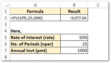
Note that, in the above example, we have kept the last two arguments [pv] and [type] as blank.
— [pv] is left as blank, as we have already specified pmt argument.
— [type] blank value denotes year end cash flows (by default)
Now, let us see how the PV function works in excel when there is monthly, quarterly, or semi-annual compounding of cash flows.
Ex. 2 – Monthly, Quarterly, Semi-annual compounding in Excel Using PV Function
Let us now see how the PV formula work in excel when investment of 1000 is made semi-annual.
I have put all the required data in the excel cells, as per below image.

To calculate the present value of cash flows that occur every 6 months (semi-annual), use the following formula:
=PV(B1/2,B2*2,B3)
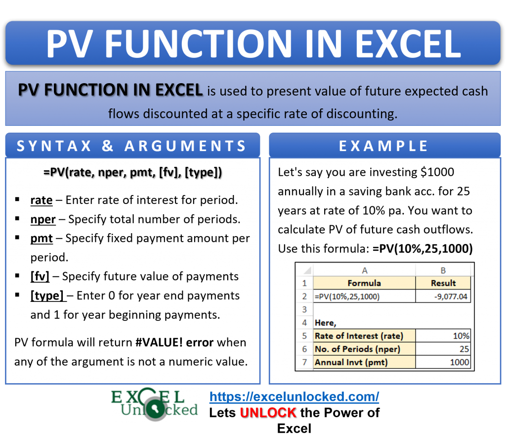
As a result, excel would return the present value as 18,255.93.
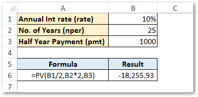
Explanation – In the above example, we have divided the annual interest rate (rate) by 2. Similarly, number of years (nper) is multiplied by 2.
This is done so as to convert present value of annual cash outflows (investment) into 6 monthly (semi-annual) cash outflows.
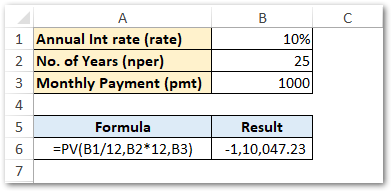
Similarly, to convert present value of annual cash flows into monthly compounding, divide and multiply the rate and nper by 12, respectively.
=PV(B1/12,B2*12,B3)
Conclusion
To convert an annual interest rate to a periodic rate, use this formula:
rate = annual interest rate / no. of periods per year
And also make sure to input the correct total number of periods:
nper = no. of years * no. of periods per year
Do Not Miss These Points
The below points are worth understanding to get a correct PV of investment and cash flows:
- The rate argument must be either in percentage (i.e. 10%) or decimal (i.e. 0.10) format only. Never put it in number format (like 10).
- If you are investing money, the money goes out. In such case, enter the pmt argument as negative value.
On the other hand, if you are receiving annuity monty, the money comes in. Therefore, enter the pmt argument value as positive value.
- PV formula will return #VALUE! error when any of the argument is not a numeric value.
Thank You 🙂
RELATED POSTS
- NPV Function – How to Calculate NPV in Excel
- Excel XNPV Function – NPV With Irregular Cash Flows
- NPER Function in Excel – Calculating Number of Periods
- PMT PPMT IPMT Functions of Excel – Usage
- ISPMT Function of Excel – Interest Amount Keeping the Principal Constant
- IRR Function in Excel – Internal Rate of Return

