The term NPV stands for Net Present Value. The Net Present Value refers to the discounting of the series of expected cash flows generated throughout the life of the project. In this tutorial, we would learn how to calculate the net present value using the excel NPV function and formula.
Let us first learn what is NPV in financial management and then deep dive into its calculation in excel. 😎
What is Net Present Value (NPV) in Financial Terms?
NPV is nothing but the present value of the future expected cash flows discounted at a specific rate of discounting minus the initial investment outlay.
The NPV is used to determine if an investment project is worth taking up or should be postponed/scrapped.
Financially and mathematically, the calculation of NPV goes like this:
NPV = Total Present value of future cash flows (PVCF) - Initial Investment

Here, PVFC = Cash Flow / (1+r)n

where, r = discounting rate ; n = year

All the PVFCs are summed up to compar with the intial outlay. If the NPV is positive, the project is worth accepting, else reject the project.
When To Use NPV Function in Excel
NPV formula in Excel is used to calculate the net present value of future cash flows with the help of excel. Many financial analysts do not use any calculator to find NPV, instead, they prefer using the NPV excel function or NPV calculator in excel.
The NPV function considers the time interval between two cash flows as equal (which is one year). Thus, any other time interval like 2 years, or quarters, or months will result an incorrect NPV value.
To calculate NPV with irregular interval cash flows, try the XNPV function in excel.
Surprising Fact About NPV Excel Function
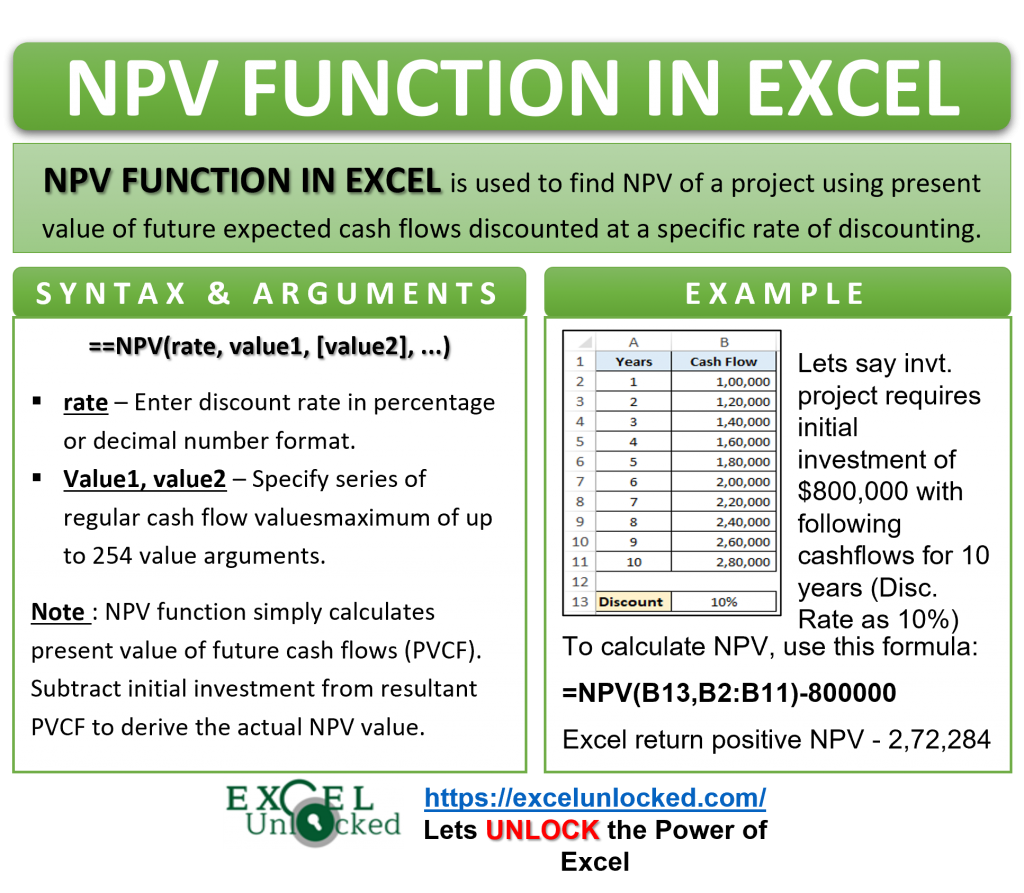
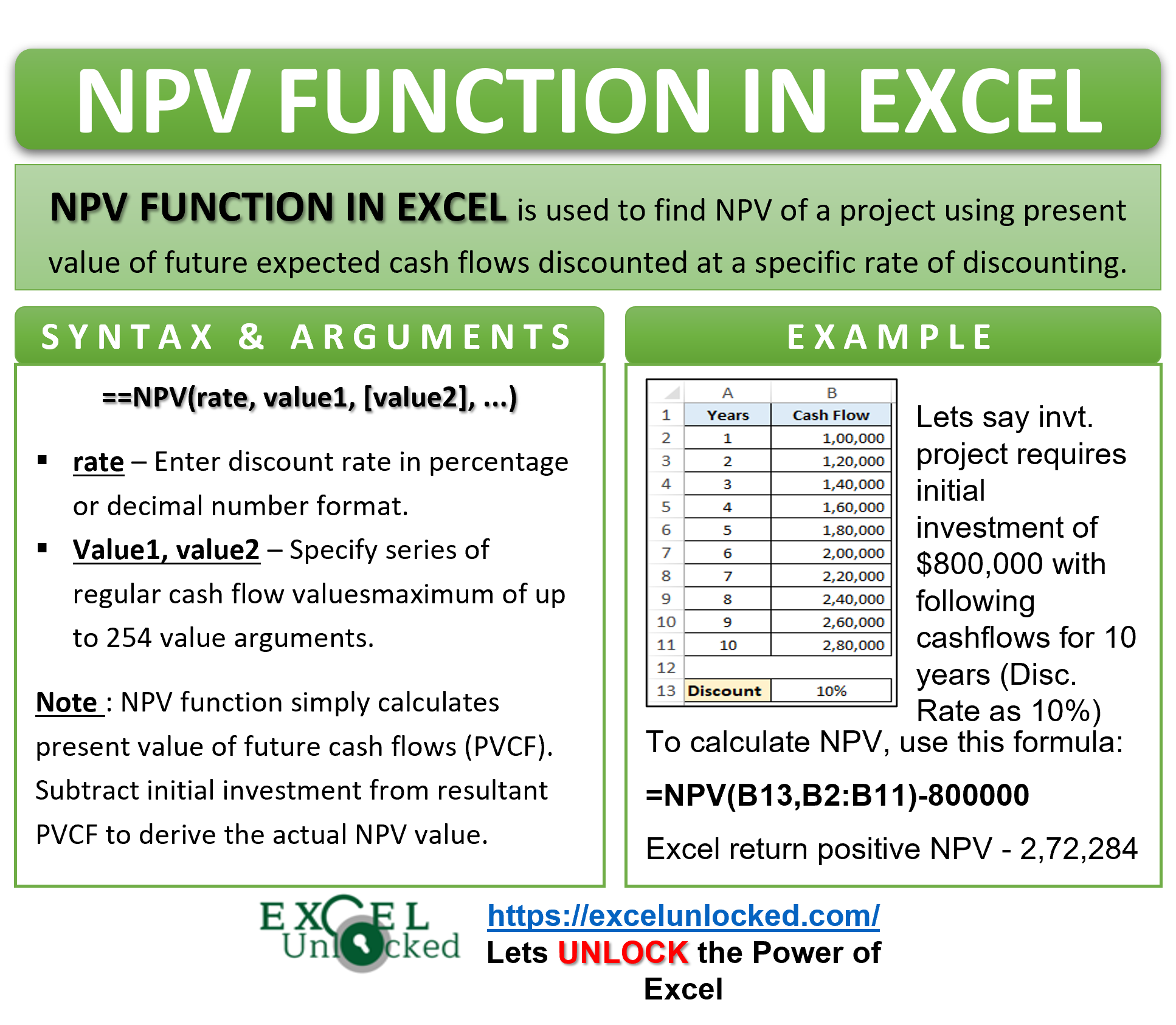
Surprisingly, excel’s NPV function does not directly calculate the net present value. Instead, it just calculates the present value of future cash flows (PVCF) component. To calculate the NPV, simply subtract the initial outlay/investment from the resultant PVCF.
=NPV(rate, value1, [value2], …) – Initial Investment Amount
Syntax and Arguments
=NPV(rate, value1, [value2], …)
The NPV excel function has the following arguments:
- rate – In this argument, enter the discounting rate.
- value1, [value2] – In this argument, specify the series of regular cash flow values. Here, value1 is mandatory and rest all values (i.e. value2, value3 and so on) are optional.
This function is available in all the excel versions. You can specify a maximum of up to 254 value arguments in Excel 2007 to modern excel versions.
Examples of Excel NPV Function
In this section of the tutorial, we would learn how to use the NPV excel formula with the help of a practical example.
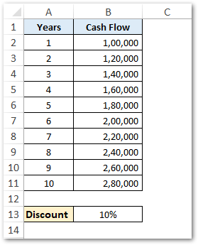
Suppose a prospective investment project requires an initial fund investment of $800,000.
Also, this investment is expected to generate the following revenue figure during its life of 10 years. Discounting factor is 10%.

For calculating NPV in excel using the above data, we need to first calculate the discounted future cash flows.
To calculate the present value of discounted cash flows, simply use the following formula:
=NPV(B13,B2:B11)
As a result, excel will return the PVCF value as 10,72,284 (rounded off).
Now, subtract the initial investment amount from the PVCF to derive the NPV of the investment proposal as shown below:
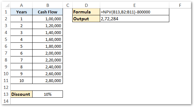
=NPV(B13,B2:B11)-800000
As a result, excel will return the NPV of the project as 2,72,284.

As a finance guy, I would conclude with this that since NPV is positive, the project is worth investing. 😉
Instead of selecting the series of cash flow values, if you wish you may even select the cash flow values individually, each separated by comms. Have a look at the below formula:
=NPV(B13,B2,B3,B4,B5,B6,B7,B8,B9,B10,B11)-800000
However, the above formula is quite complex to understand and can accept a maximum of 254 value arguments.

Do Not Miss These Points
To make sure that the NPV excel function returns a correct value, it is important to keep the following points in mind before using the NPV function for your project appraisal.
- The future cash flow must occur at the end of the respective years, and not at the beginning of the year. Therefore, in the above example, the cash flow of $100,000 is assumed to have occured at the end of year 1. Similarly, cash flow of $240,000 is assumed to have occured at the end of year 8.
As a result, we need to adjust the initial investment amount of $8,00,000 outside the NPV function.
- The NPV function considers the series of values in a chronological order. It means in range B2:B11 (above example), cell value B2 represents year 1, cell value B3 represents year 2, and so on.
- To display a cash flow outflow, use negative value (i.e with minus sign before the value).
- Any value other than numeric value (in the series) are ignored, such as empty cells, errors codes, etc.
- The discounting rate must always be entered in either percentage (say 10%) or a decimal format (0.10). Never simply write the numeric value to represent discount rate (E.g. 10). For excel NPV formula, 10 means 1000%. This would result into incorrect NPV value.
Thank You 🙂
RELATED POSTS
- FV Function of Excel – Find Future Value of Investment
- NPER Function in Excel – Calculating Number of Periods
- IRR Function in Excel – Internal Rate of Return
- Excel RATE Function – Calculating Interest Rate for Specified Period
- PMT PPMT IPMT Functions of Excel – Usage
- MIRR Function in Excel – Modified Internal Rate of Return

