PMT PPMT IPMT Functions of Excel – Usage

The PMT, PPMT, and IPMT functions in excel are the three financial formulae in excel. These three function are quite related to each other. While taking any loan, you may be choosing which loan works best for you. What would be the interest? Does the loan provider charges weekly interest rate, monthly interest rate, or annual interest. What is going to be the interest amount that I would be paying once the loan is paid? All these questions will be answered by the combination of PMT, PPMT and IMPT formula in excel.

Let us see how these functions works. Here we go 😎

When to Use PMT, PPMT, IPMT Function of Excel

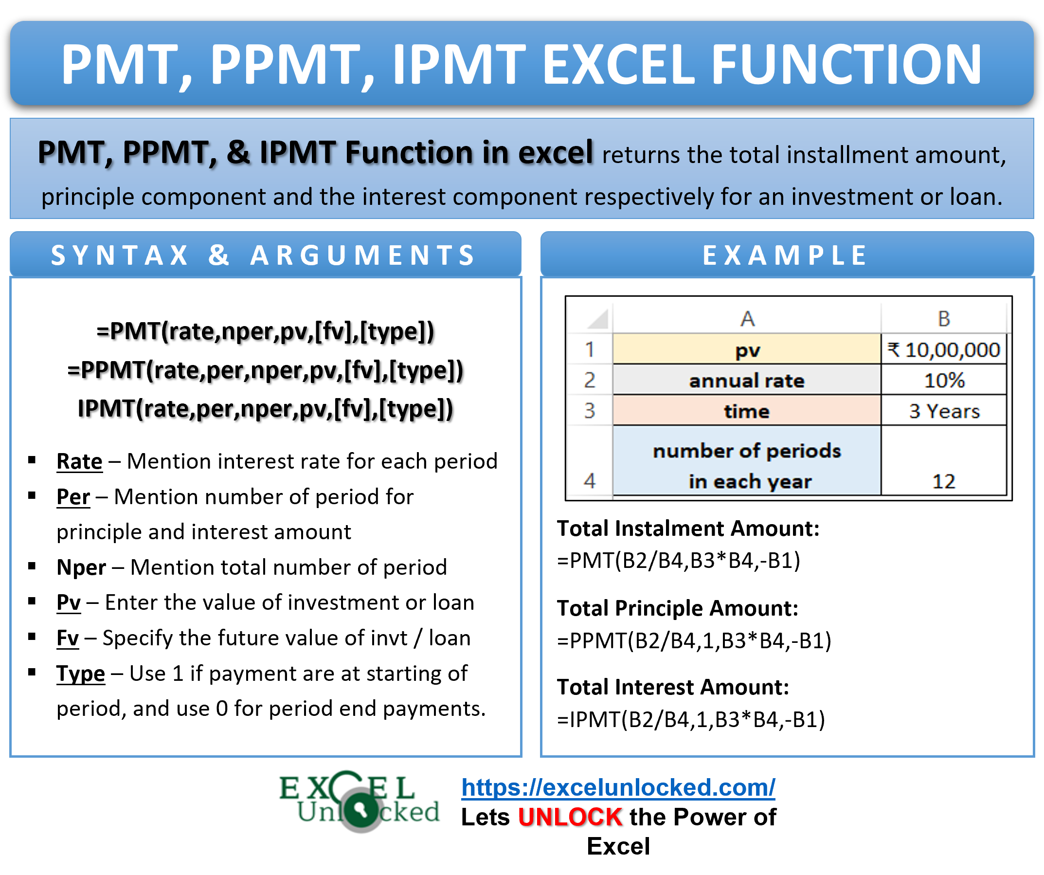
The word PMT stands for “payment” for each period. The PMT function of Excel gives the total payment (principal amount + interest money) which we need to pay when taking a loan or we receive on investment.

The word PPMT stands for “Principal Payment” for each period. The PPMT function of Excel gives the principal amount of money from the total payment transacted at the end or beginning of the period. If we took a loan, then the Interest amount will start decreasing with the coming periods whereas the principal amount is paid more to get the loan settled. This concept is explained in more details in the upcoming examples.

The word IPMT represents “Interest Payment”. The IPMT function of excel returns the amount that will be paid as interest. When we take a loan, we return the principal amount with the interest money in the coming periods. The interest lowers down as the money we took for a loan is getting returned in installments, reducing the amount on which we are paying the interest money.

The three functions are a part of Financial Functions of Excel.

Syntax and Arguments

The following are the syntax for PMT, PPMT, IPMT formula in Excel.

=PMT(rate,nper,pv,[fv],[type])

=PPMT(rate,per,nper,pv,[fv],[type])

=IPMT(rate,per,nper,pv,[fv],[type])

Below are the function arguments Explained.

• rate – This is the interest rate for each period.

• per – This is the number of period for which we want to get the principal payment (PPMT) or interest payment (IPMT)

• nper – This represents the total number of periods.

• pv – It is the present value of the loan or investment.

• fv – This is an optional argument representing the future value.

• type – When we are making payments at the starting of each period, then the type is 1. This leads to less interest and principal amount as you are returning the loan amount earlier when compared with the payment being done at the end of each period (type = 0).

You must have noticed that the PMT function does not require per function argument. This is so because :

Payment (PMT) = Principal (PPMT) + Interest (IPMT)

Must Remember – Excel PMT, PPMT, IPMT Function

The following points must be kept in mind before actually using these functions.

• The value of per argument for PPMT and IPMT function must lie between 1 and nper (total number of periods).

• The money is negative for cash outflow whereas it is positive when money received.

• Default value of type is 0.

• We might need to change the annual interest rate into quarterly, monthly or weekly interest rates.

• nper can never be zero or negative value.

• The default value of fv is 0.

Examples for PMT, PPMT and IPMT Functions of Excel

In this section of the blog, we will discuss some examples to get practical knowledge of these functions.

Ex.1 – Simplest Usage of PMT, PPMT and IPMT Functions

Let us say that there is an investment of rupees 10,00,000 by a business at a constant annual interest rate of 10%. The money is for a period of 3 years.

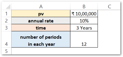
We want to know the monthly payment, the principal amount, and the interest earned for the first period only. We are going to use the following formulas respectively.

=PMT(B2/B4,B3*B4,-B1)

=PPMT(B2/B4,1,B3*B4,-B1)

=IPMT(B2/B4,1,B3*B4,-B1)

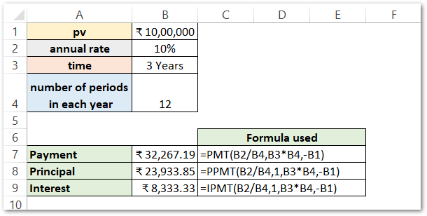
As a result, the formula returns a total installment amount for each period as 32,267.19.

The Principal and Interest for the first period are 23,933.85 and 8,333.33, respectively.

We can verify this using the following arithmetics:

Installment (32,267.19) = Principal (23,933.85) + Interest (8,333.33)

Explanation – The annual interest rate is 0.1 or 10%. There is a total of 12 periods in the year each year. The interest rate for each period becomes B2/B3.

There contains 12 periods in one year and the time period is of 3 years. The total number of periods or nper becomes B4*B3.

B1 contains the present value of the loan.

per is a required function argument for PPMT and IPMT functions. Consequently, the value of per is 1 for the first period.

However, the values of fv and type are default values (0).

Ex. 2 – Getting Monthly Payment, Principal and Interest Amount for Each Period of Loan

In this example Let us say Ms. Mehta took a Loan of Rs 5,00,000 from the bank at an annual interest rate of 12.50% for 1 year. There is a total of 12 periods in each year. Below is the data.

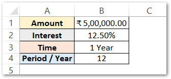
Getting Periodic Payment- PMT

We will use the following PMT formula to get the payment, Ms. Mehta has to pay at the end of each period.

=PMT(B2/B4,B3*B4,B1)

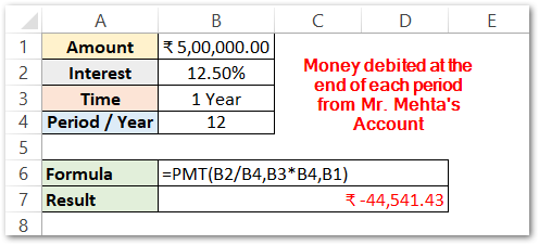
As a result, the PMT formula has returned the periodic payment debited for each period.

Explanation – The annual interest for the loan is 12.50% which converts to the periodic interest rate. There are a total of 12 periods in a year. The periodic interest rate becomes 12.50/12% or B2/B3. The total number of periods is the product of the Total number of years and the number of periods per year. In other words, we can say that nper is B3*B4. Whenever there is an outflow of cash, there comes a negative sign before money i.e -B1, where B1 is the loan amount.

The result is negative value as the money withdraws as the payment each month.

Getting Principal Amount for 12 Periods – PPMT

We will now calculate the principal amount of money that Ms. Mehta will pay from the periodic payment.

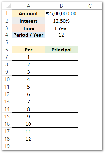
Use the following formula to get the principal amount from each payment in cell B7.

=PPMT($B$2/$B$4,A7,$B$3*$B$4,$B$1)

As a result, the PPMT function has returned the principal amount (rs 39,333.10) for the first period. We have used the excel fill handle tool to get the principal amount for each period.

We have used absolute referencing for cell B1,B2,B3 and B4 so that when we copy down the formula, these cells remain locked. The per input argument (A7) is in relative referencing so that the principal amount is calculated for different periods when the formula copies.

Explanation – We have the same function arguments that we passed to the PMT formula. There is one extra input argument per that represents the period number for which we want to know the principal amount. The range A7:A18 contains the n number of periods.

Getting Interest Amount for Each Period – IPMT

We will now use the IMPT function to know that how much money from the payment is the interest amount. Use this IMPT Formula to get the results.

=IPMT($B$2/$B$4,A7,$B$3*$B$4,$B$1)

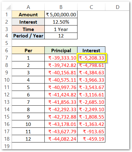
As a result, the formula has returned the interest amount for the first period as rs 5,208.33. We have copied the formula to get the interest amount at the end of each period.

Result Verification – PMT PPMT IPMT

As we know that the payment calculated by PMT is constant for every period as rs 44,542.43

We can now get the sum of the total principal amount, interest amount, and payment by using the SUM Function of Excel.

=SUM(B7:B18)

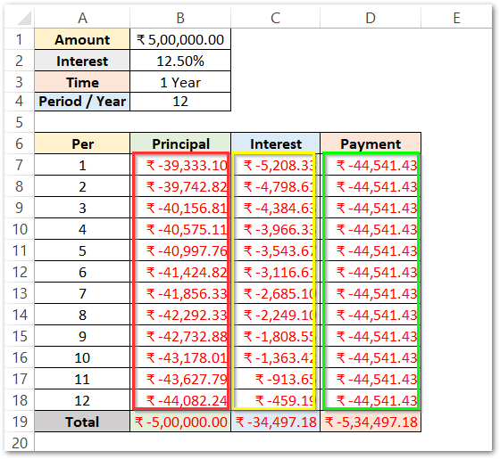
As a result, we can now see that the sum of the principal amount in cell B19 is the total loan amount that Ms. Mehta took. The total interest for 12 periods comes out to be rs 34,497 on the loan.

The sum of principal and interest amount is giving the payment amount for each period as well as for the total of 12 periods. Consequently, this also verifies the equation.

Payment = Principal + Interest

Here we come to the end of PMT PPMT and IPMT Functions of Excel. Thank you for reading 😉