Excel RATE Function – Calculating Interest Rate for Specified Period

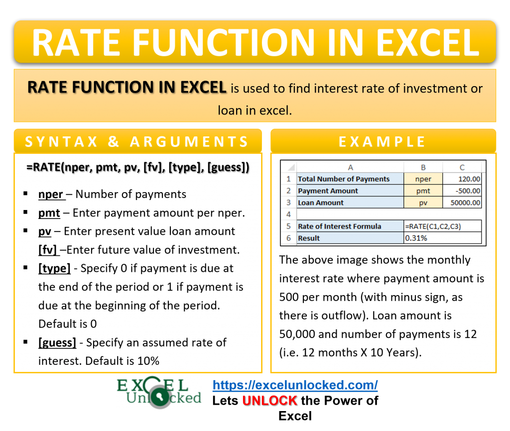
When you apply for any loan (home loan, car loan, etc.) from the bank, the first and foremost thing is to calculate the interest rate or amount on the loan. Similarly, you may have to find and calculate the return on investment (ROI) rate on the investment made. The excel financial functions are very useful in such cases when you want to know how to calculate interest rate in excel. In this tutorial, we would learn one such formula called the RATE function in Excel.

Here we go 😎

When To Use RATE Function in Excel

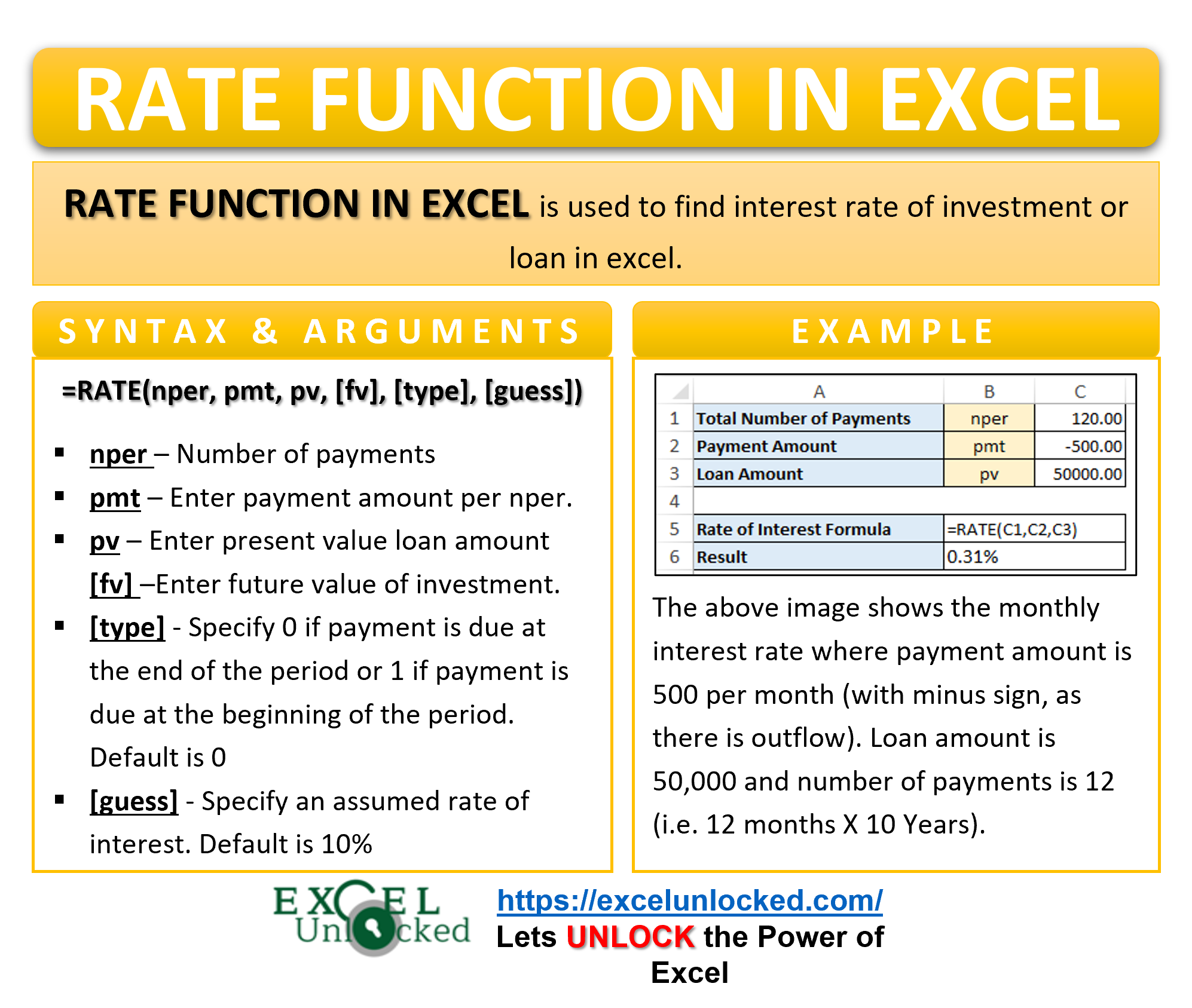
The RATE formula in excel is used to find the rate of interest charged on a loan in excel given the specified period. Similarly, it may be useful to calculate the return earned on the investment. This function belongs to the Financial formula excel group.

The RATE function is very useful for calculating the interest rate on saving bank account, fixed deposit (FD), etc.

Syntax and Arguments

=RATE(nper, pmt, pv, [fv], [type], [guess])

The function has six arguments (three mandatories and three optional):

• nper – In this argument, specify the number of interest/loan payment periods (month, year, week, etc.)

• pmt – In this argument, specify the payment amount per period. It is important to note that this amount must be fixed one. It includes both interest and principle component.

• pv – It stands for present value. In this argument, specify the loan amount i.e. present value of investment.

• [fv]– It stands for future value. In this argument, specify the future value (i.e. future amount that you want to have after the end of all the periods). If it is left blank, it is assumed as zero (0).

• [type] – This argument accepts two values – 0 and 1. Specify 0 if payment is due at the end of the period or 1 if payment is due at the beginning of the period. If this argument is left empty, it is assumed as zero (0) i.e. due at the end of period.

• [guess] – In this argument, specify an assumed rate of interest, based on your knowledge. If it is left blank, it is assumed as 10%.

Do Not Miss These Points

• It is important to note that you must specify a positive numbers for cash inflows and negative numbers for cash outflows. Incorrect usage of positive and negative numbers will return #NUM! error (discussed later in this tutorial).

• Although the pv argument is required (mandatory), you may keep it as blank if you specify fv argument. (See example 4)

RATE Formula in Excel – Example

Let us look at some simple examples to understand how to make the RATE formula in excel.

Ex. 1 – Calculating Monthly Interest Rate in Excel

In this first example about the Excel RATE formula, let us learn how to find and calculate the monthly interest rate using excel function.

Let say, you have availed loan of $50,000 and as per the agreement with the bank, interest payments are monthly for 10 years. Monthly payment amount $500.

• The total number of payments (nper) will be 120 (i.e. 12 X 10).
• pmt will be -500.
• Loan amount (pv) will be 50000.

It is important to note that since there is an outflow of money, the pmt figure will be a negative figure (with a minus sign before the number).

Use the following formula to calculate interest rate in excel with the above values:

=RATE(120,-500,50000)

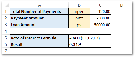
As a result, excel returns the rate of interest as 0.31%. Note that the interest rate of 0.31% is a monthly interest rate.

Ex. 2 – Calculate Annual Interest Rate in Excel

In this section, we would learn how to calculate the annual interest rate in excel if you already have the monthly interest rate.

Continuing with the above example, calculating the annual interest rate in excel goes like this.

To calculate the annual interest rate, simply multiply 12 to the monthly interest rate:

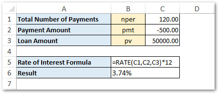
 =RATE(120,-500,50000)*12

Ex. 3 – Calculate Quarterly Interest Rate in Excel

Similarly, to calculate the quarterly interest rate, multiply the monthly interest rate by 4, as shown in the below image.

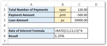
  =RATE(120,-500,50000)*4 

Ex. 4 – Calculate Interest Rate When You Know Future Value

In all the above examples, we learned how to calculate interest rate when you know present value. In this section, we would cover how to find interest rate when you know future value and not present value.

Let’s say you want to have maturity amount of $100,000 at the end of 10 years by investing 500 per month on periodic basis.

In this case, we have the future value with us (viz. 100,000). To find the interest rate, simply us the following formula:

=RATE(120,-500,,100000)

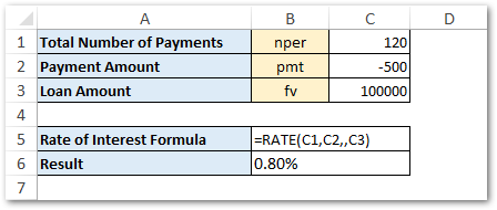
As a result, excel would return 0.80% as monthly rate of interest.

The annual rate of interest will therefore be 9.58% (0.80 X 12) calculated using this formula:

 =RATE(120,-500,,100000)*12

RATE Formula Returns Negative Interest Rate Percentage (Incorrect)

If you get a negative rate of interest percentage or the RATE function return incorrect output (a higher or lower rate than expected), then probably you have missed converting the number of years into the total number of payments (nper argument).

To resolve this issue, make sure to pass the correct nper argument value.

To reiterate, the nper argument represents the total number of payments and not the total number of years.

nper for monthly payment = years * 12

nper for quarterly payments = years * 4

Likewise, nper for semi-annual payments = years * 2

RATE Formula Return Zero Percentage (0%) in Excel

Many times, the RATE function may return an incorrect result, such as 0%.

No need to panic about the result. It is simply a number formatting issue. The reason for the 0% RATE formula result is because the value is less than 1%.

To resolve this, simply use the ‘Increase Decimal’ button (Home tab > Number group > Increase Decimal) and see the magic 😉

#NUM! and #VALUE! Error in RATE Function Excel

The RATE function may return excel formula error like #NUM! and #VALUE!. Below sub-sections explain the reason and probable solution.

#NUM! Error by Excel RATE Formula

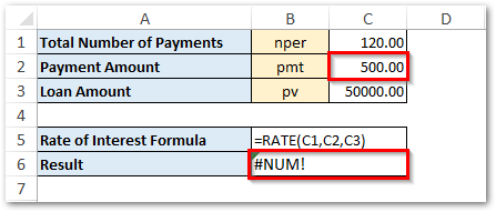
Reason – The most probable reason for #NUM! error in RATE function is an incorrect usage of values. For example, if you do not specify a negative number (with minus sign) for outgoing payments, RATE formula returns #NUM! error.

Similarly, by putting a minus sign for incoming payments, will return #NUM! error.

#VALUE! Error by Excel RATE Formula

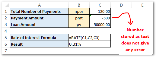
Reason – The #VALUE! error occurs in RATE function when you specify a non-numeric value for any of the formula arguments.

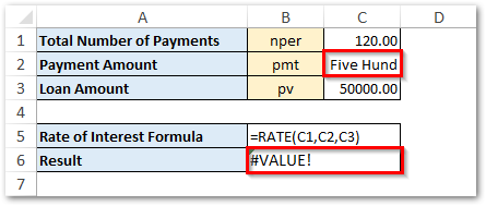
It is important to note that, the number formatted and stored as the text will not bother the output of the RATE function, as shown in the below image.

Thank you for reading 🙂