AVERAGE Function in Excel – Finding Mean or Average Value in Excel

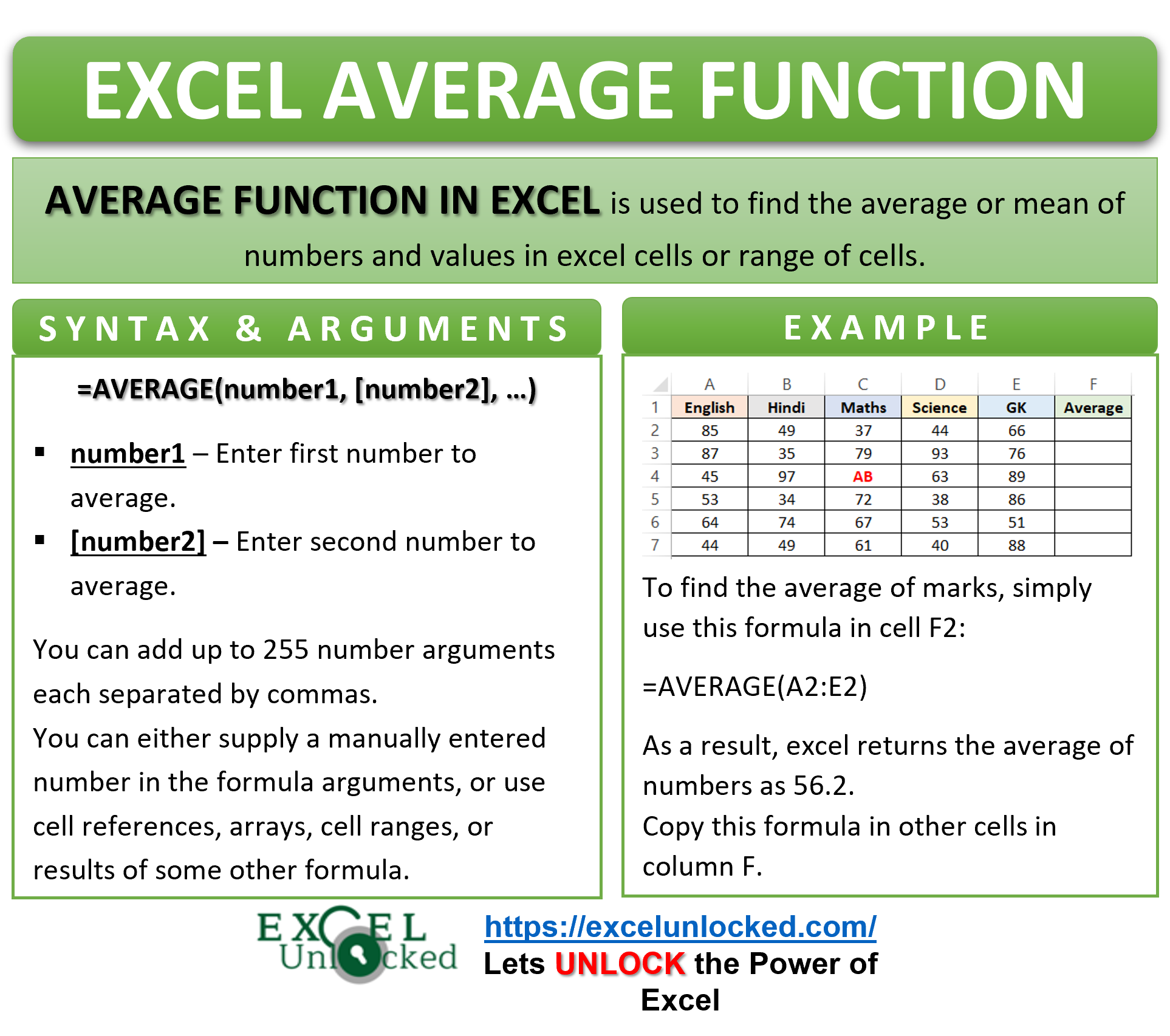
In this tutorial, we would learn how to find the mean of values and numbers using the Excel AVERAGE function.

Here we go 😎

When to Use AVERAGE Formula in Excel

As the name suggests, the AVERAGE function in excel is used to find the average of numbers, values, etc. It is a powerful statistical inbuilt function in excel.

We can easily find the mean value of numbers, dates, time, currencies, or cells having any other numerical format.

When we need to find the average marks of five subjects of a student or the average sales of laundry for one month, the AVERAGE function comes into its use.

Points to Know About AVERAGE Function in Excel

The following points are important to know before going to syntax and arguments.

• The function ignores blank cells and cells containing text strings.
• AVERAGE formula in excel ignores Logical values (TRUE or FALSE).
• The function will count the cell containing a zero in the total number of numerical values. For instance, when you apply AVERAGE formula on cells containing 10, 20 and 0 it would be 10 (i.e. 10/3) and not 15 (10/2).
• We can use AVERAGE function with ROUND function in excel, to get a rounded off average value with specified number of digits after decimal point.
• AVERAGE function can find the avergage scores of top 3 students by taking LARGE function in Excel as the function arguments.
• If we pass only logical values, the function would give a #DIV/0 error.
• If we pass only text strings to AVERAGE formula, it will return a zero.

Now, we will study the syntax and arguments for the Excel AVERAGE formula

Syntax and Arguments

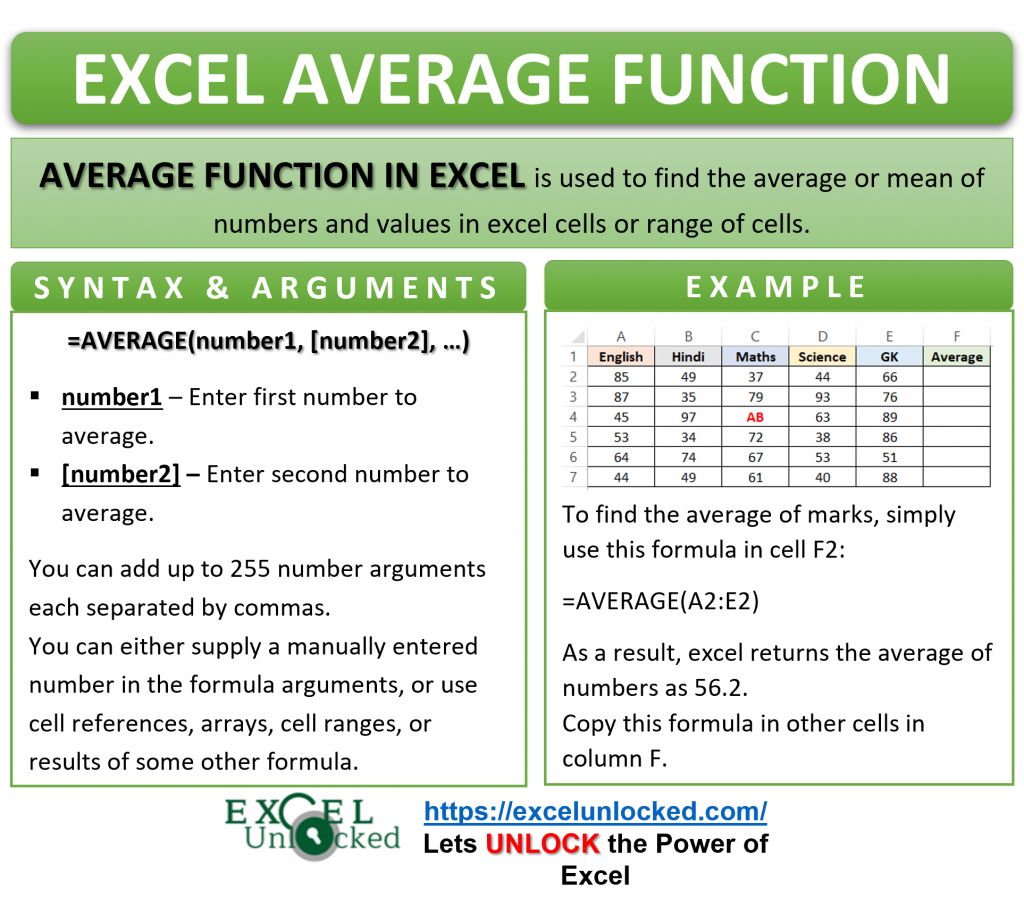
=AVERAGE(number1,[number2]……..)

• number1 – In this argument, enter the number, cell refrence, range , blank cell or a function to find the average for.
• [number2] – This optional argument accepts same values linke number1.

There can be 255 arguments in the AVERAGE function of excel. The first argument is a compulsory argument, while the other 254 being optional.

Examples To Learn AVERAGE Formula in Excel

In this section of the blog, we have some useful examples for finding the mean result.

Ex. 1 – Passing First Argument to AVERAGE Function in Excel

Firstly, let us start by taking the annual marks of students. We are going to use the AVERAGE function to find the average marks of each of the students.

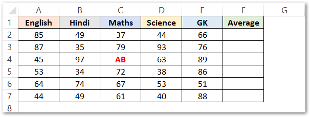
Enter this formula in cell F2 to get the average marks of the first record.

=AVERAGE(A2:E2)

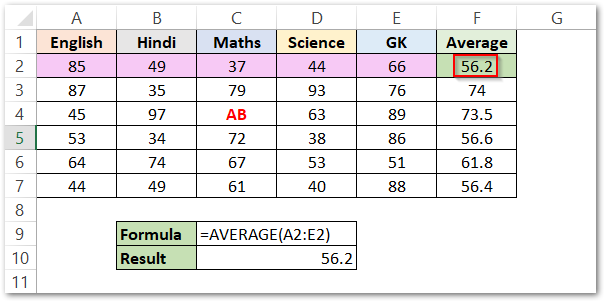
As a result, excel returns the average of numbers as 56.2.

Explanation – In the above formula, we pass the range A2:E2 containing the first record of marks. The AVERAGE function returned the average marks of a student in five subjects in cell F2 as its result.

Copy the formula to other cells in column F.

In the third record, one student is marked absent by a text string “AB” in cell C4. The AVERAGE formula is copied successfully in cell F4, with cell C4 ignored as it has a text string.

Ex. 2 – Passing Multiple Arguments To AVERAGE Function in Excel

In this example, we will be passing multiple arguments to the AVERAGE formula in Excel.

For instance, we have taken three cell ranges as given below.

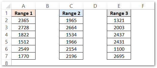
Use the AVERAGE formula as mentioned below to find the average value of the data contained in three ranges.

=AVERAGE(A2:A7,C2:C7,E2:E7)

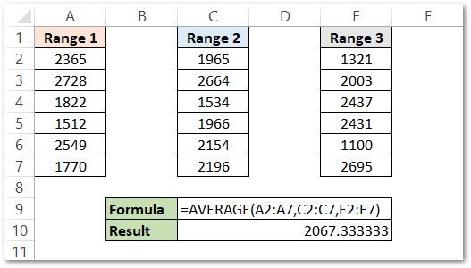
As a result, the function has returned 2067.333333 as the mean of three ranges.

Explanation – We have passed three cell ranges A2:A7, C2:C7, E2:E7. The function has returned the mean value of the data contained in the three ranges to be 2067.333333. We can also round off the result to get a whole number value by using the Excel ROUND Function.

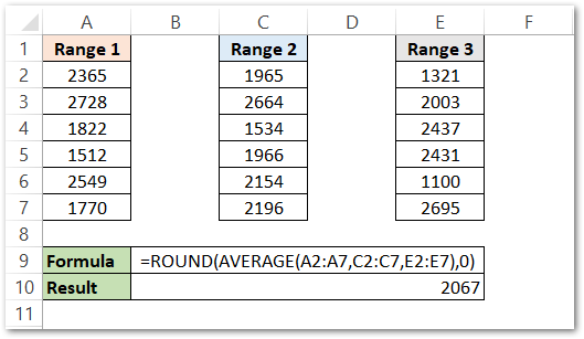
In the above formula, we have used the ROUND function with the AVERAGE function in Excel. Consequently, the function has rounded off the result of the AVERAGE formula to zero decimal places.

Similarly, we will now be using the LARGE function of Excel with the AVERAGE formula to see how it works.

Ex.3- Using AVERAGE Formula With LARGE Function in Excel

Below are the monthly sales of a company for one year.

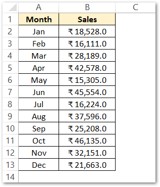
Use this formula to find the average of the top three monthly sales of the year.

=AVERAGE(LARGE(B2:B13,{1,2,3}))

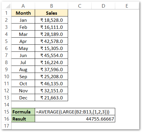
As a result, the function has returned 44755.66667 as the average of the top three sales.

Explanation – Firstly, we will try to understand the fact that this time we have passed a function to the AVERAGE formula argument. The large function is the function argument of the AVERAGE function. The LARGE function has returned the top 3 values from the range B2:B13 to the AVERAGE formula. After that, the AVERAGE function has calculated its mean.

Ex. 4 – Using AVERAGE Formula of Excel With Dates

At last, we will now try this formula to find the mean value of dates.

Below are the subscription details of different customers of a company package. The subscription for the first month is free, but when half of the free month subscription has passed, the customer has to purchase a yearly package from the company which will be automatically activated once the free subscription ends.

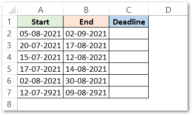
We will now use the AVERAGE formula to find the deadline for payment of the yearly package (halfway between starting and ending of free one-month subscription ) for each of the customers.

=AVERAGE(A2:B2)

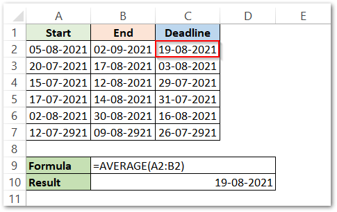
As a result, the function has returned the deadline as 19-8-2021 for the first customer.

Explanation – The AVERAGE formula used in cell C2 has successfully calculated the deadline of payment that lies between the date in cells A2 and B2. We can easily copy the formula by simply double-clicking the bottom right corner of cell C2 or by dragging the mouse to the bottom for rest of the subscription records.

Congratulations! You have now learned enough for the AVERAGE function in excel.

Thank you for reading 🙂