RANK.AVG Function in Excel – Usage, Error Handeling

In the previous blog, we learned about the RANK Function. RANK.AVG function in excel is an updated version of the RANK Formula. RANK.AVG function was introduced in Excel 2010 and can be used in later versions.

Let’s work on learning the RANK.AVG function in Excel.

When to Use RANK.AVG Function in Excel?

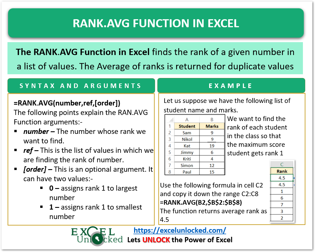
RANK.AVG function in excel gives us the rank of a numerical value in a list of values.

If any numerical value is repeated more than one time, then the function returns the average of their ranks. The RANK.AVG function can work in two different ways:-

• Descending order (Default):- In this mode, the ranks are assigned as if the list of values is arranged in descending order of values. Moreover, the largest value is assigned with rank 1. For Example:- A student scores the first rank in class if he has the highest marks.
• Ascending order:- In this mode, the ranks are assigned as if the list is arranged in increasing order. In other words, we can say that the first rank is given to the minimum value. For example, A runner has scored the first rank if he completes the race in minimum time ( smallest value of time ).

RANK.AVG function is one of the important Statistical Functions in Excel.

Syntax and Arguments

=RANK.AVG(number,ref,[order])

Where the following list contains the required information for RANK.AVG Function arguments.

• number – This is the value whose rank we want to find. It can be a hardcoded value or reference to a cell containing the numerical value.
• ref – This is the range containing a list of all numerical values. In comparison, we get the rank of the number in this list.
• [order] – This argument specified the mode for the arrangement to get ranks. It is an optional argument and is not mandatory to specify. It can be:-
  • 0 – (descending order) This is the default value. It assigns the first rank to the largest value.
  • 1 – (ascending order) It assigns the first rank to the smallest value.

Examples to Learn RANK.AVG Function in Excel

In the following section of the blog, we would learn the practical usage of RANK.AVG function in excel to find rank via examples. Let’s get started with it!

Example 1 – Assigning Ranks to Class Students in a Test

In this example, let us suppose we have the marks of students in a class test as follows:-

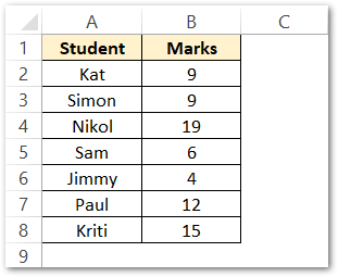
Moreover, you need to notice one thing, Kat and Simon both scored 9 marks on tests. We will use the following RANK.AVG formula in cell C2 and copy it down the range C2:C8:-

=RANK.AVG(B2,$B$2:$B$8)

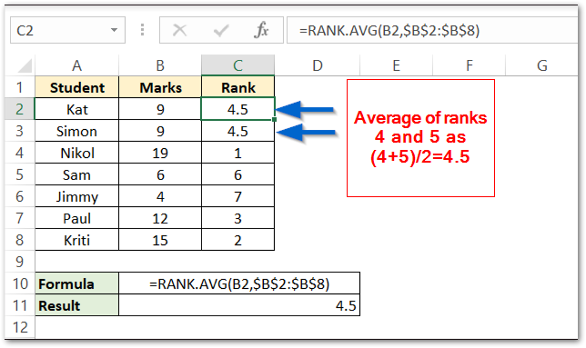
As a result, you can see that the RANK.AVG has assigned ranks to each of the students as per their marks.

Explanation:- We have passed cell B2 as the number because we want to look at the rank of this number. The locked range $B$2:$B$8 passes as a ref argument because it contains the list of entire class marks. We did not specify the order argument which is why the function used the default value i.e 0

We can make the following conclusions from the RANK.AVG function results:-

• Nikol got the first rank because of her highest marks of 19.
• Kat and Simon have equal marks. In other words, we can say that there are duplicate values as 9 repeats two times in the marks list. RANK.AVG takes the average of their ranks. If Kat and Simon did not score equal marks then one of them would be at rank 4 and the other at rank 5. The function takes the average rank as 4.5

Example 2 – Finding Ranks as per Increasing Order ( Ascending Order )

In this method, the first rank allots to the smallest value. Let us suppose we have the list of time taken by different runners to complete a 1 KM round.

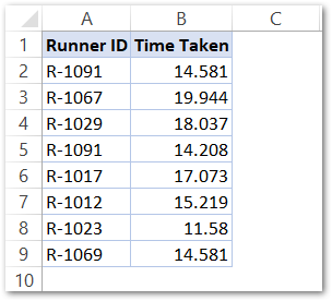
We want to find the rank scored by different runners so that the runner who took the minimum time to complete the race gets the first rank. Use the following formula in cell C2 and copy it down the range C2:C9.

=RANK.AVG(B2,$B$2:$B$9,1)

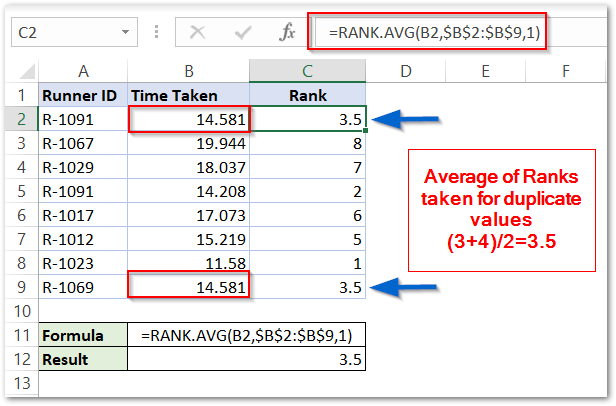
As a result, you can see that the formula has successfully returned the ranks of all runners.

Explanation – We have passed cell B2 as the number argument of the RANK Function as it has time taken by each runner. We supply the range B2:B9 to ref argument as the list of different time values. We pass 1 in the [ order] argument so that the data sorts in ascending order. Rank 1 assigns to the minimum value.

We can make the following conclusions for the runner’s ranks:-

• R-1023 scored the first rank as it took a minimum time to complete the race i.e 11.58 minutes
• Exception – As the First and last runner on the list took equal time to complete the race, the average of their ranks is returned by the RANK.AVG formula

Important Points to Remember About RANK.AVG formula

The following points about the RANK.AVG function must be kept in mind for its execution.

• The RANK.AVG returns a #N/A! error if the number argument is not present in the list or the number is any text string.
• RANK.AVG function cannot be used in excel 2007 and earlier.
• RANK.AVG ignores the non-numerical values supplied in the ref argument.
• The function returns a #VALUE! error if the number is any logical value.

Consequently, we have reached the end of the blog.

Thank you for reading.