RANK Function in Excel – Usage with Examples

The RANK Function is one of the most easiest and useful excel functions. In this blog, we would learn the syntax and arguments required by the RANK Function along with its practical usage.

So let’s start working.

When to Use RANK Function?

As the name “RANK” suggests, the RANK Function gives the rank of a particular value in a list of different numerical values. In the backend ( we cannot see it),

• the RANK Function sorts the list of numerical values either in ascending ( smallest first ) or in descending ( largest first ) order.
• The Smallest number is assigned with Rank 1 when the list of values is sorted in ascending order.
• The Largest number is assigned with Rank 1 when the list of values is sorted in descending order.

The RANK Function returns a #N/A error when the number whose rank we want to find, does not exist in the list of values.

RANK Function comes under the category of Statistical Functions in Excel.

Syntax and Arguments

=RANK(number,ref,[order])

The following points explain the required function arguments to successfully operate the RANK Formula:-

• number – This is the value whose rank we want to find.
• ref – This is a reference to a list of values in which we want to find the rank of number. The list need not be sorted.
• [order] – This is an optional argument, asking whether we want the list of values to be in ascending orders or in descending order. It can be:-
  • 0 – This is the default value. It assigns the rank 1 to the largest number ( descending order ). For example, to find the rank of a student in a class test
  • 1 – This assumes the list to work in ascending order. The smallest value is assigned with rank 1. For example, a Bike racer that took the minimum time to complete the race will be ranked highest.

Examples to Learn RANK Function in Excel

In this section of the blog, we will be learning some of the practical examples to better understand the working of the RANK Formula in Excel.

Example 1 – Finding Rank as per Decreasing Order (default mode)

Let us suppose we have the list of students with their corresponding marks in a class test as follows:-

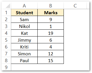
Here we want to know the rank scored by each student in the class assuming that rank 1 is assigned to the highest marks in the class. In other words, we can say that the minimum rank will be assigned to students with greater marks.

Use the following formula in cell C2 and copy the formula down the range C2:C8 using the Excel Fill Handle tool.

=RANK(B2,$B$2:$B$8)

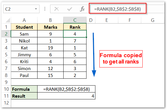
As a result, you can see that the formula has returned the corresponding ranks of students.

Explanation – We have passed cell B2 as the number argument whose rank we want to know. Here B2 cell contains the corresponding student marks. The list of marks B2:B8 is supplied as the ref argument. The range $B$2:$B$8 contains the list of marks that are locked ( absolute referencing in excel ) so that it does not change when the formula copies down the range C2:C8.

We can make the following conclusions from the student ranks.

• Kat scored the highest of 19 marks and thus got first.
• Nikol scored the lowest 1 mark which is why she got 7th rank which is equal to the total students appearing for the test.
• Paul and Simon scored second and third positions in the test respectively.

Example 2 – Finding Ranks as per Increasing Order ( Ascending Order )

In this method, the first rank allots to the smallest value. Let us suppose we have the list of time taken by different runners to complete a 3 KM round.

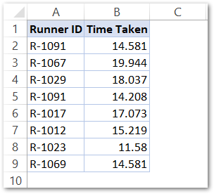
We want to find the rank scored by different runners so that the runner who took the minimum time to complete the race gets the first rank. Use the following formula in cell C2 and copy it down the range C2:C9.

=RANK(B2,$B$2:$B$9,1)

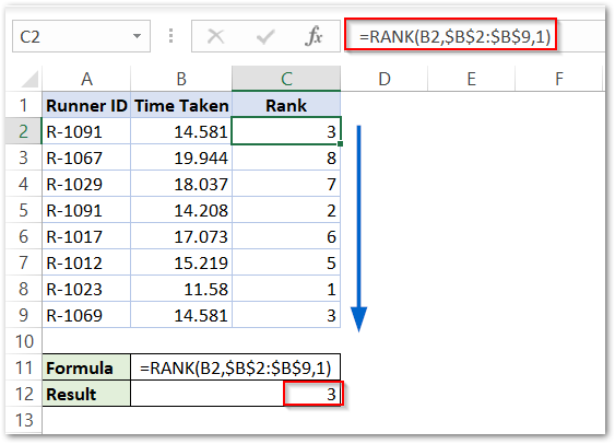
As a result, you can see that the formula has successfully returned the ranks of all runners.

Explanation – We have passed cell B2 as the number argument of the RANK Function as it has time taken by each runner. We supply the range B2:B9 to ref argument as the list of different time values. We pass 1 in the [ order] argument so that the data sorts in ascending order. Rank 1 assigns to the minimum value.

We can make the following conclusions for the runner’s ranks:-

• R-1023 scored the first rank as it took a minimum time to complete the race i.e 11.58 minutes
• Exception – No runner scored Rank 4. This is so because Runners R-1091 and R-1069 ( first and last runners on the list) took an equal time of 14.581 minutes to complete the round. This is why both the runners were assigned with the third rank. The next runner R-1012 scored rank 5.

Important Points to Remember about RANK Function

We must remember the following points about the RANK Function for its successful implementation:-

• RANK Function returns a #N/A! error in two situations:-
  • The given number is not present in the referred list.
  • We use the text representation of numbers in the function arguments.
• Logical Values supplied to the RANK function, make it return a #VALUE! error.
• RANK.AVG and RANK.EQ function has replaced the usage of the RANK Function in Excel.

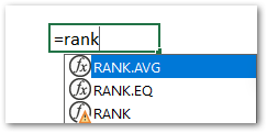
The RANK Function comes with this Warning symbol. This is so because the function is available for compatibility with Excel 2007 and earlier. But we can use it successfully in newer versions also.

This leads to the successful completion of the blog. Thank you for reading.