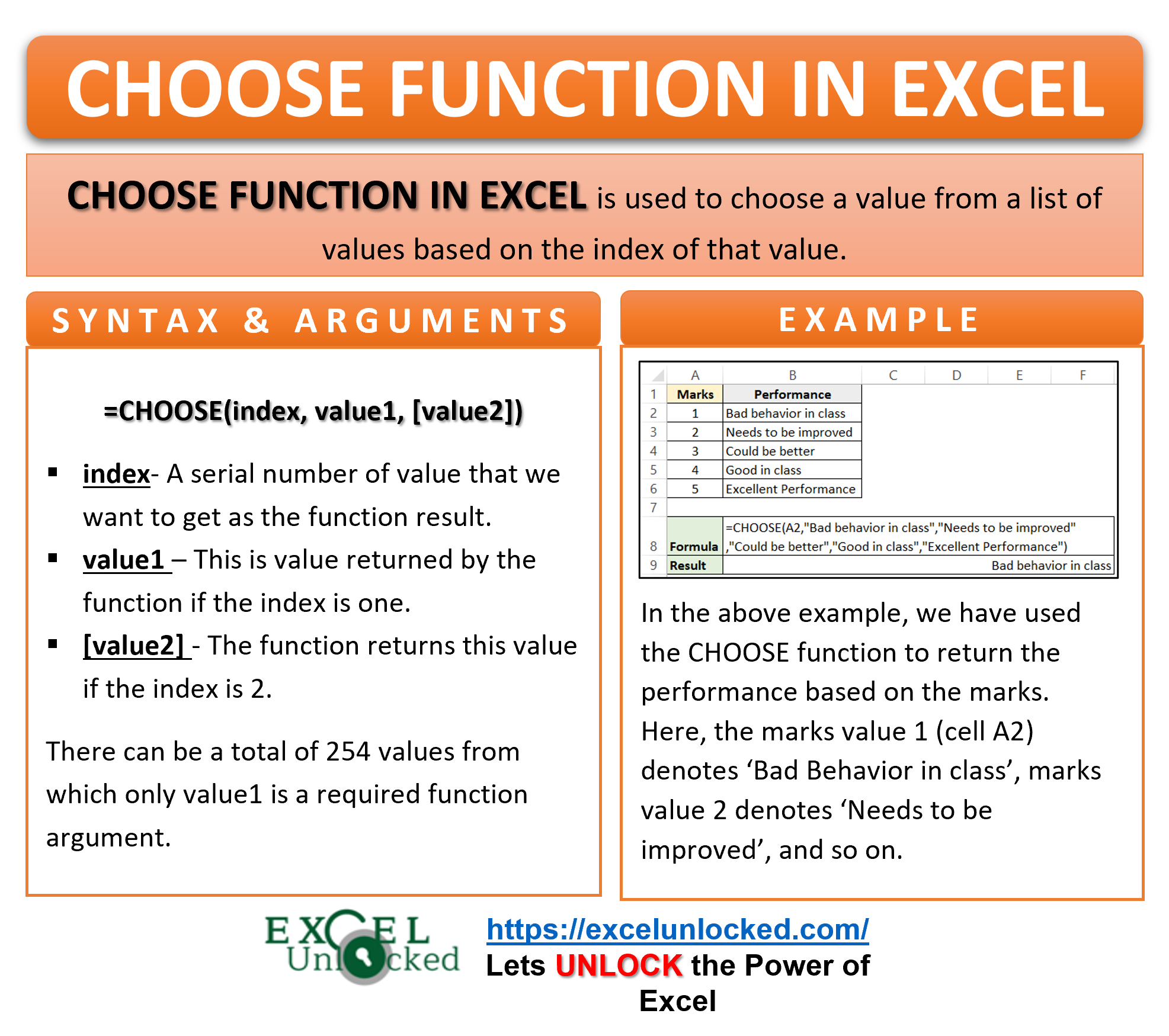
The CHOOSE function is a very powerful function of Excel. The function is used in many cases like creating raw data for dashboards, to get month from dates, etc. Let us see the usage of this function.
Here we go 😎
When to Use CHOOSE Function of Excel
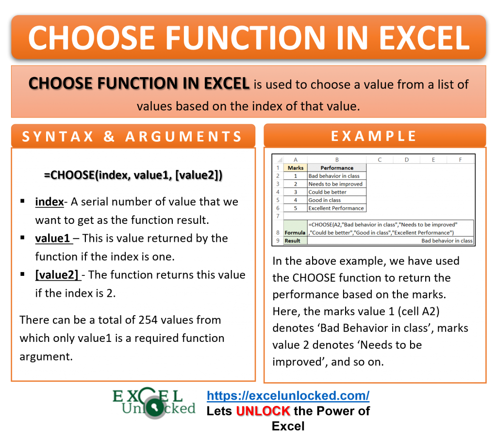
The CHOOSE function is used to choose a value from a list of values based on the index of that value. The function returns the value that corresponds to the index or the serial number of that value.
The CHOOSE Function can be categorized under the Lookup and Reference Functions of Excel.
Syntax and Arguments
=CHOOSE(index, value1, [value2])
The below points will explain to you the required function arguments for CHOOSE Function of Excel.
- index – It is the serial number of the value that we want to get as the function result. It can be a serial number or an array of numbers.
- value1 – This is the value returned by the function if the index is one. It can be a number, text string, a formula, cell reference or a range of cells.
- [value2] – The function returns this value if the index is 2. This is an optional argument.
There can be a total of 254 values from which only value1 is a required function argument.
Must to Know Points About CHOOSE Function in Excel
The following points must be kept in mind before actually using the CHOOSE Function of Excel.
- The function returns value1 if the index is 1, value2 if the index is 2, value3 if the index is 3 and so on.
- This function can also be used as an array function to return a value that can be a range of cells . ( check example 3)
- The CHOOSE Function returns a #VALUE! error if there is no value that corresponds to the index number. For instance =CHOOSE(2,1), in this formula the index is 2 but the value2 is not specified, making the function to return a #VALUE! error.
- The function goes well, even when there are extra value arguments with their index numbers not specified. For instance, look at this formula =CHOOSE(RANDBETWEEN(1,3),1,2,3,4). Here the index can be 1, 2, 3 but there are four value arguments as 1, 2, 3, 4.
Examples to Learn CHOOSE Function in Excel
In this section of the blog, we will go through some examples to learn the usage of CHOOSE function of Excel.
Ex.1 – Simplest Example for CHOOSE Formula
In this example, let us say that there are the student marks for class performance that are rated from 1 to 5. Below are the marks:-
Also Read: N Function in Excel – Usage and Examples
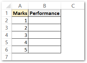
We want to mark the performance as per the marks given to the students for class performance. Use the following CHOOSE Formula to get the results.
=CHOOSE(A2,"Bad behavior in class","Needs to be improved","Could be better","Good in class","Excellent Performance")
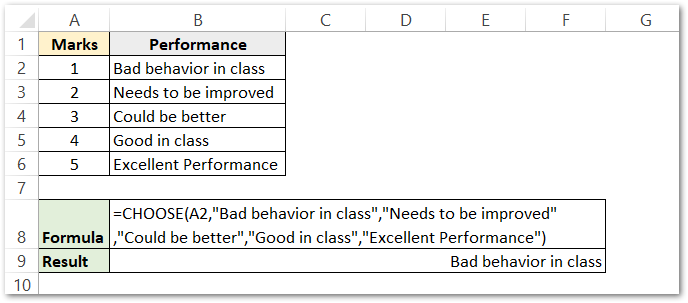
As a result, the function has returned a text string “Bad behavior in class” in cell B2. We have used the Excel fill handle tool to copy the formula to the rest of the cells.
Explanation – In this function, the index is A2, In other words, the index is 1. As we know when the index is 1, the function returns value1. Value1 is a text string “Bad behavior in class”. So the function has returned a text string “Bad behavior in class” when the mark is 1.
Similarly, when we copy the formula in cell B3, the index becomes A3 or 2. The function returns Value2 as “Needs to be improved” to be the formula result.
Also Read: TYPE Function in Excel – Get Data Type
The function would return “Could be better”, “Good in class”, and “Excellent Performance” when the marks (index) are 3, 4, 5, respectively.
Ex.2 – Returning Month Name from Dates using MONTH Function with CHOOSE Formula
Let us day in this example, we have the data of a company that contains the manufacturing dates of different products. We want to add a column that specifies the month of manufacturing for each of the products. Below is the data.
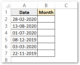
We will use the following CHOOSE Function ( in cell B2) with the MONTH Function of Excel to get the results.
=CHOOSE(MONTH(A2),"Jan","Feb","March","April","May","June","July","Aug","Sep","Oct","Nov","Dec")
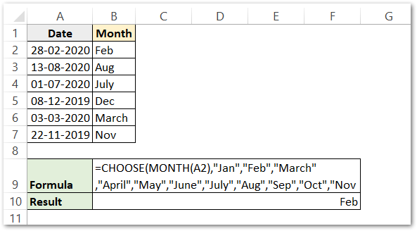
As a result, the formula has returned the month to be Feb for the date 28-02-2020. We have copied down the formula for the rest of the manufacturing dates.
Explanation – We have defined the index of CHOOSE Function as the result of the MONTH function of Excel. The MONTH Function extracts the number of months from the date. In this example, the date in cell A2 is 28-02-2020, so the month becomes 2. The result of the MONTH Function becomes the index for CHOOSE formula. If the index is 2, then the CHOOSE Formula returns value2. In other words, the Formula returns a text string “Feb”.
Similarly, when the MONTH Function returns 1,2,3,4,5,6,7,8,9,10or 12, then the CHOOSE function returns corresponding values as “Jan”,”Feb”,”March”,”April”,”May”,”June”,”July”,”Aug”,”Sep”,”Oct”,”Nov or “Dec”.
Ex.3 – Using the CHOOSE Function As Array Function
In this example, let us say that below is the data for Railway Booking System. There are two columns representing the name of the train and ticket availability.
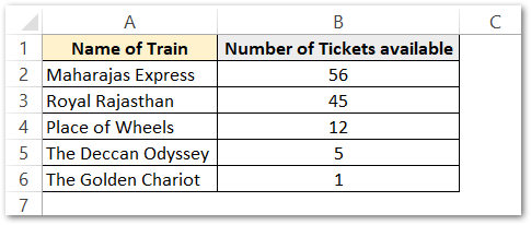
We want to apply the VLOOKUP formula to get the ticket availability for the trains. Use this formula in cell B9.
=VLOOKUP(A9,CHOOSE({1,2},A2:A6,B2:B6),2,0)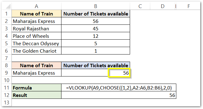
Now If you type the name of the ticket in cell A9, the formula will return the number of tickets available for that train in cell B9. As a result, the formula has returned 56.
Explanation – In the above VLOOKUP Formula, the lookup value is set to A9. In other words, the function will search this in the lookup array. The Lookup array is returned by the CHOOSE Function of Excel. There is a list of index numbers as {1,2} which will return both the value1 and value2. Value1 is the range A2:A6 (train names) while value2 is B2:B6 (Tickets available). So the lookup array becomes A2:B6. The column index is 2 which means that the second column from the lookup range will contain the result as of the corresponding lookup value. When we looked for “Maharaja Express”, in the lookup range A2:A6, the formula returned the corresponding number of tickets for it from B2:B6.
Thank you for reading 😉

