The COLUMN function in excel is a part of the reference functions which find the reference of cell in Excel. In this blog, we would learn one of these reference excel functions which is the COLUMN formula in excel.
This tutorial would cover about what is the use of the excel COLUMN function, its syntax, arguments, and examples.
What is Use of COLUMN Function in Excel
The purpose of the COLUMN excel function is to return or get the column number of the selected cell or any other specified cell in Excel.
The result of COLUMN formula in Excel is a whole number (1, 2, 3, 4 … and so on).
Syntax and Argument
=COLUMN([reference])
There is only one argument of the excel COLUMN formula.
- [reference] – This is the optional argument of the COLUMN function. In this argument, enter the reference of the cell of which you want to find the column number.
Since the argument is an optional argument, therefore if you keep it as blank, the formula would return the column number of the active cell (i.e. cell in which the formula exists).
Examples
Let us consider both types of examples of excel COLUMN formula.
Using Column Excel Function (without argument)
As mentioned earlier, the only argument of this function is also an optional argument. So, if you keep the argument blank, excel would return the column number of the active cell.
Enter the following formula in the cell of which you want to get column value in Excel.
=COLUMN()
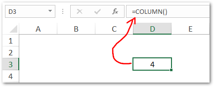
Suppose, I want to get it for cell D3. Therefore, I have entered the above formula in cell D3.

As a result, excel returns the whole number 4. This is because column D is the fourth column in the Excel worksheet.

Using Column Excel Formula (with Argument)
To get the column number of some other cell in Excel, simply give a reference of that other cell as input argument as shown below:

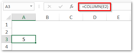
In the above example, I have found the column number of cell E2 (i.e. 5) inside cell A3 by using following formula:
=COLUMN(E2)
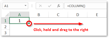
The column function is very useful when you want to get the sequence of numbers (1,2,3,4,…) from left to right in a row. Simply type =COLUMN() in cell A1 and then use the excel fill handle tool to drag it to other cells to the right.

As a result, the =COLUMN() formula would copy to the cells to the right and return the column number of the individual cells (B1, C1, D1, and so on).

