Similar to the COLUMNS formula, the ROWS function in excel is also one of the excel reference formulas used to find the cell references.
In this tutorial, we would learn about the excel ROWS formula, its syntax, and its argument with examples.
Here we go 😎
When to Use Excel ROWS Function
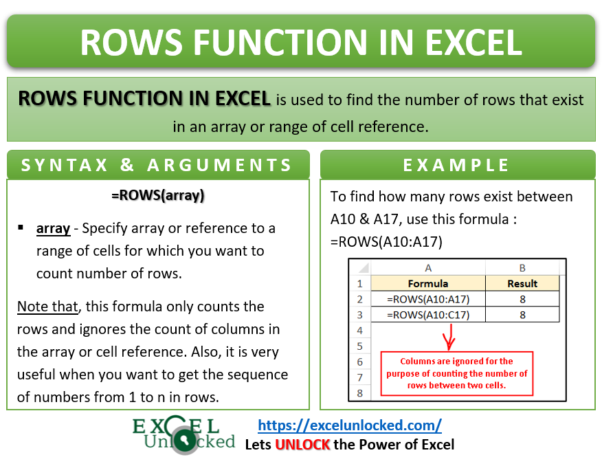
The ROWS formula in excel is a useful function to find and return the number of rows in excel within a cell range or cells array. It assists you to get the count of rows between two cells in excel.
As an output of this function, you would get a whole number like 1, 2, 3, 4, and so on.
Syntax and Argument
=ROWS(array)
The ROWS formula only supports one input argument which is ‘array’.
- array – In this argument, mention the range of cells or an array value to count rows in excel.
Example of ROWS Formula in Excel
Let us start with a very basic example of how the ROWS formula works in excel to understand its usability.
Also Read: ROW Function in Excel – Get Cell Row Number
By using the ROWS function in excel, finding the number of rows between two excel cells becomes very easy.
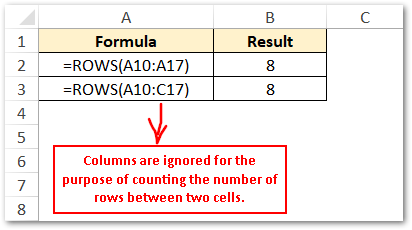
Suppose you wish to find about how many rows exist between two cells A10 and A17. To achieve this, simply use the following formula:
=ROWS(A10:A17)
As a result, excel returns the whole number 8. This means there are 8 rows in between cells A10 and A17.
See the image below for better understanding.

Do Not Miss This Point
It is important to consider the following point regarding excel ROWS formula.

- This formula simply counts the number of rows that come up in between two cells and therefore ignores the columns. Let us consider cells A10 to C17. As a result of the formula =ROWS(A10:C17) you would notice that excel again returns 8 as formula output. The columns A to C are ignored over here.

Practical Usage of ROWS Excel Function
Initially, I was wondering on how is the ROWS formula used practically.
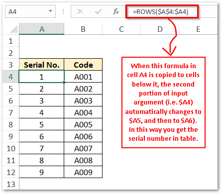
Later on , in one of my projects, I realized its importance. Using the ROWS excel formula, you can find the return sequence or serial number in an excel table very easily. See the image below:

In the above image, the formula in cell A4 is =ROWS($A$4:$A4). When this formula is copied to cells A5, A6, and so on, the second $A4 in the input argument changes to $A5 and $A6 as so on. This results in getting the sequential serial number in the excel table.
