INDEX Function in Excel – Get Intersection Point

The INDEX function in excel is one of the highly used excel formula to fetch particular data from a table based on the row and column number.

In this tutorial, we would unlock how the INDEX formula in excel works along with its syntax, arguments, and examples.

So let us begin 😎

When to Use Excel INDEX Function

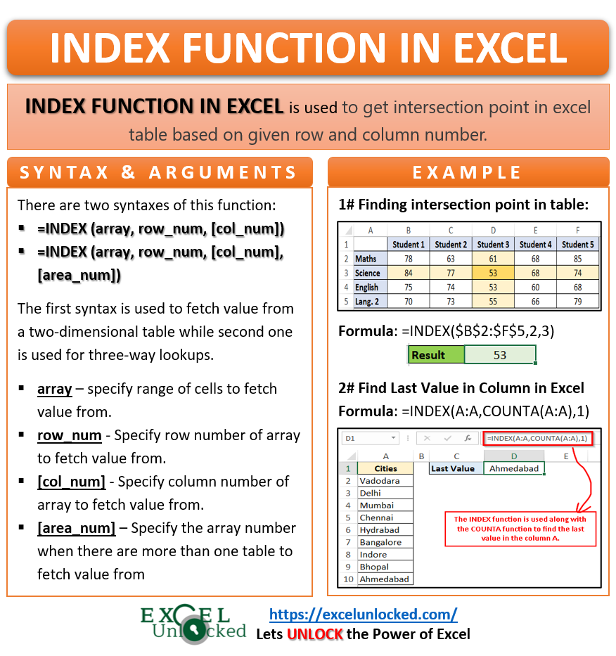
The excel INDEX formula is an amazing function that is useful to get the intersection point in the table based on the given row number and the column number. It is useful to fetch a particular value from table data.

See the image below for understanding:

In the above diagram, the INDEX excel formula helps in finding the intersect value ’53’ for the rows and columns in excel.

Syntax and Arguments

Unlike the other excel formulas and function, the INDEX formula has two syntaxes.

• =INDEX (array, row_num, [col_num])

• =INDEX (array, row_num, [col_num], [area_num])

How the Two Formula Syntaxes Differ?

• The first syntax is useful to fetch the value from the two-dimensional table (i.e. two-way lookup).
• The second one is useful for three-way lookups in the table.

In majority of real-life excel scenarios, the first formula syntax helps.

Let us now discuss about the four arguments of the INDEX formula:

• array – In this argument, specify the range of cells from which you want to fetch the value. In the case of tabular data tables, specify the cell range excluding the header rows and columns.

• row_num – In this argument, specify the row number from which you wish to fetch the value.

• [col_num] – This is an optional argument. In here, specify the column number from which you want to get the value.

• [area_num] – This argument is used when there are more than one tables and you want to fetch value from a specific table from it using the row and column number.

INDEX Function Examples in Excel

Now, when you are aware of the purpose of the INDEX excel formula and its syntaxes and arguments, it’s time to take one basic example to understand how the INDEX function works in excel.

1# How to Find Intersection Point in Excel Using INDEX function

Let us take the example shown above:

To find the marks obtained by ‘Student 3’ in ‘Science’, simply use the following formula:

=INDEX($B$2:$F$5,2,3)

As a result excel would return the value 53.

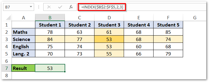
Explanation of the above formula – In the above formula the range $B$2:$F$5 denotes the area from which you want to get the value. The row_num 2 and the col_num 3 specifies the row and column number from the range $B$2:$F$5 to fetch value from.

2# Find Last Value in a Column in Excel

Using the INDEX function along with the COUNTA formula is helpful in finding the last value in the column in excel.

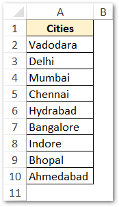
In the below image, columln A consist of the names of Indian cities. Now, we want to find what is the the last value in this column.

To achieve it, use the following formula:

=INDEX(A:A,COUNTA(A:A),1)

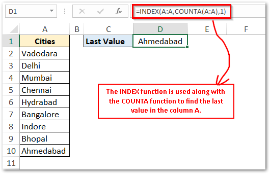
Explanation of the above formula – In the above formula, the COUNTA(A:A) function tries to find the number of rows which has a value in range A:A. As a result, the COUNTA(A:A) results 10, as there are 10 rows in column A that are filled with some values. Finally, the INDEX function returns the value in the 10th row (which is Ahmedabad).

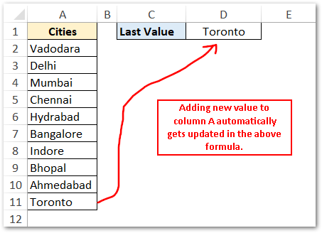
Now, if you add any new city in the 11th row, the formula would automatically update. See the illustration below:

Do Not Miss These Points

• Generally, the INDEX formula is not used on its own. It is used along with other functions like COUNTA (learned above), MATCH, etc. to enhance its functionality.

• The INDEX function has an added advantages of looking for values from right to left of the data table. This is not possible in other lookup functions like VLOOKUP.

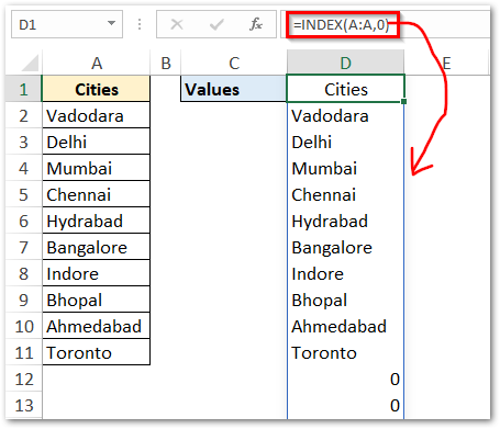
• If you keep the value of row_num or col_num arguments as 0 (zero), then the INDEX excel function returns values of the entire row or column. See the image below:

You can increase your learning by going through the powerful application of INDEX and MATCH Function of Excel – LOOKUP using the INDEX and MATCH formula.

Thank You 🙂