HLOOKUP Function in Excel – Match Value in Row

The HLOOKUP function in excel is another lookup excel formula that is used to find and get value from a table based on another value. It works similarly to the VLOOKUP Excel function.

In this tutorial, we would unlock everything about the excel HLOOKUP function, its syntax, arguments with examples.

When to Use HLOOKUP Function in Excel

The excel HLOOKUP formula is a lookup excel function that is used to find a particular value or text in the row based on another value in the table.

To put in simple terms, the HLOOKUP excel formula searches for a particular text/value in a specific row in excel and if it finds that text/value in that row, then it returns another corresponding value based on that value/text.

This is the reason why some people call HLOOKUP as Horizontal LOOKUP.

Understanding Excel HLOOKUP Function with Example

The below image shows the sales value achieved by five sales representatives in 12 months of the year.

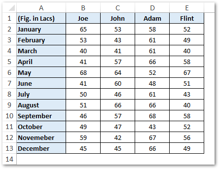
Now, suppose you want to find the sales value achieved by ‘Adam’ in the month of August. How would proceed?

You can use either of these two approaches to achieve this:

• You can first move down in column A to search for the month ‘August’, and then move to the right 4 columns to get value for Adam. This is exactly what the VLOOKUP excel formula does.

OR

• The second approach is to first move to the right to search for the name ‘Adam’ and then go down by 9 rows to get the value for the month of August. This particular approach is exactly how the HLOOKUP formula functions in excel.

Now when you have a thorough understanding of how the HLOOKUP function works in excel, let us deep dive into the excel HLOOKUP function.

Syntax and Arguments

=HLOOKUP(lookup_value, table_array, row_index_num, [range_lookup])

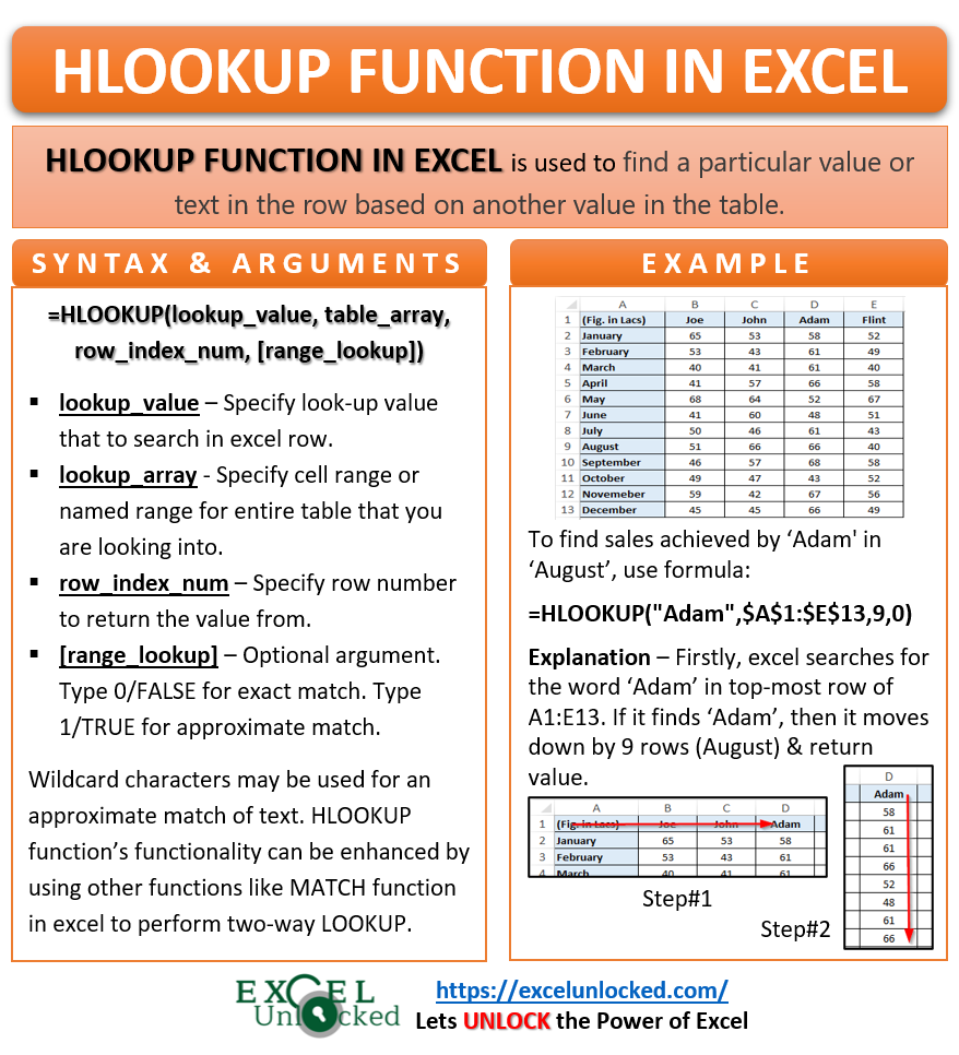
• lookup_value – Mention the value that you want to find in an excel row from left to right. In the above example, the lookup_value is ‘Adam’ in row 1.

• table_array – Specify the entire cell range in which you are looking for the values. In the above example, the table_array is range $A$1:$E$15. This argument also accepts the named range.

• row_index_num – Specify the row number from which you want to return the value. In the sales example above, since we want to extract value for August from the table, the row_index_number will be 9. This means excel shall extract value from the 9th column in the table_array.

• [range_lookup] – This is an optional argument. In this argument, specify the match type. Use 0 (zero) or FALSE to perform an exact match of the lookup value. Or use the match type 1 (one) or TRUE performs an approximate match of values.

Simple Example of HLOOKUP Excel Formula

In this section of the blog, we would learn in detail how the HLOOKUP formula works in excel by taking one simple example.

From the data in the below image, let us find the sales value achieved by ‘Adam’ in the month of ‘August’ using the HLOOKUP function in excel

Use this formula-

=HLOOKUP(“Adam”,$A$1:$E$13,9,0)

As a result, excel returns 66, which denotes the sales achieved by Adam in the month of August.

Explanation of HLOOKUP Formula Working:

Let us now understand working of HLOOKUP function in excel.

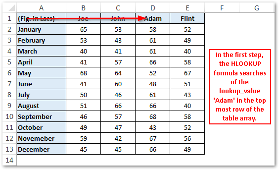
Firstly, the formula searches for the word “Adam” (first input argument) in the top-most row of the table array (range) $A$1:$E$13.

As soon as it finds the lookup_value ‘Adam’, then it moves down up to the 9th column (row_index_num) and returns the corresponding value.

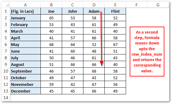
As a result, it gives output as 66.

Instead of entering ‘Adam’ as text in lookup_value input argument, you can also use a cell reference, like this:

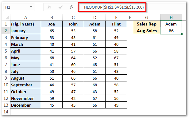
=HLOOKUP($H$1,$A$1:$E$13,9,0)

Do Not Miss These Points

• The HLOOKUP excel function return #N/A error if it does not find the lookup value in the table.

• To allow the HLOOKUP function to perform an approximate match of values (1 or TRUE), it is important that the lookup_value row is sorted in ascending order from left to right. Otherwise, the formula would return an inaccurate result.

• Another way of performing an approximate match of values in HLOOKUP is by using the wildcard characters (* and ?).

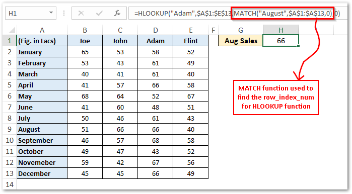
• You can also enhance the utility of the HLOOKUP formula by inserting other excel functions like MATCH function. Using the MATCH function, you can find the row number (row_index_num) using the formula.
  
  =HLOOKUP(“Adam”,$A$1:$E$13,MATCH(“August”,$A$1:$A$13,0),0)

Thank You 🙂