VLOOKUP Function in Excel – Lookup Formula

The VLOOKUP Function in Excel is an essential type of Lookup Formula. You can’t be an excel expert until you know how to implement the VLOOKUP Function. So let’s begin the process of becoming an excel expert by learning the VLOOKUP Function fundamentals.

When to Use VLOOKUP Function?

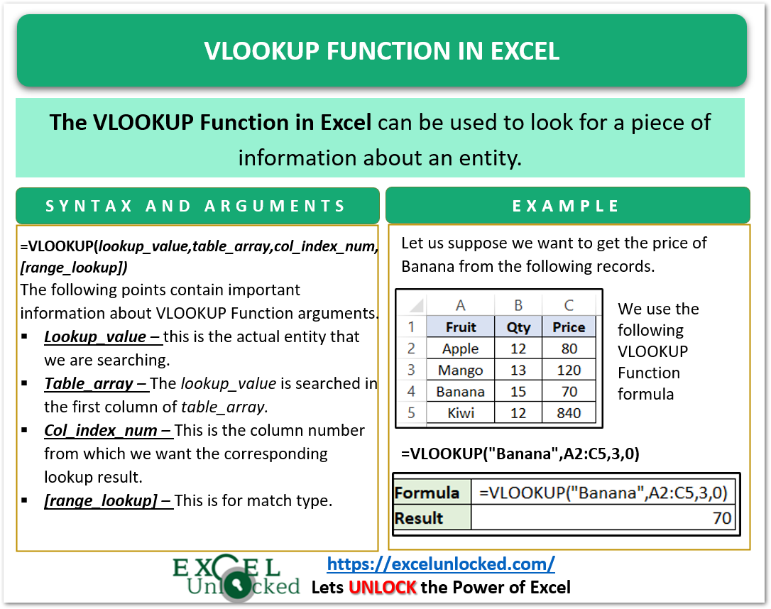
The word “VLOOKUP” stands for Vertical Lookup. The VLOOKUP Function helps us to get a particular sort of information regarding an entity from different data records. For example, I have different fruit sales data. With the use of the VLOOKUP Function, We can search for a Banana ( entity ) and get the price of the Banana ( Piece of Information ).

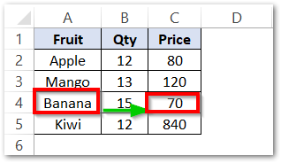
This is called a Vertical Lookup since we looked for the entity Banana in the Fruits Column ( Vertical ) and then the price of the banana ( Price Column ) is our Lookup result.

Syntax and Arguments

=VLOOKUP(lookup_value,table_array,col_index_num,[range_lookup])

The below points contain the necessary inputs required by the VLOOKUP Function in Excel.

• lookup_value – This is the entity about which we want to get the piece of information.
• table_array – This contains our data records. The function searches for lookup_value in the first column of table_array.
• col_index_num – This is the column number from which the corresponding value of the lookup_value would be returned. i.e Price column ( 3rd ) in the Fruit Sales Data.
• [range_lookup] – This is an optional argument. It tells the type of search for the lookup_value in the first column of table_array. It can have two values.
  • TRUE (Default Value)- Approximate match. If there is no value that matches with the lookup_value then the closest match lower than the closest match lower than the lookup_value is used.
  • FALSE – This represents the exact match. If there is no exact match of lookup_value, then the VLOOKUP Function would return an error.

Implementing the VLOOKUP Function in Excel

In this part, we are actually going to implement the VLOOKUP Formula. Let us suppose we have the following student records in a class.

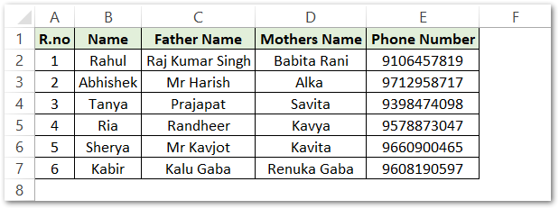
So you can see that we have the records of six students. For understanding purposes, we have taken only 6 records. There can be a larger number of records in which the lookup is not possible without the help of any LOOKUP Function like VLOOKUP.

Now let us suppose we want to find his Phone Number of Kabir.

Here Kabir is an entity and we want to look for his phone number (a piece of information )

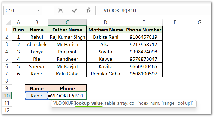
Step 1 – Specifying the Lookup Value

Here, we want to get the phone number of Kabir. We will take cell B10 to contain the name of the student whose information we want to find.

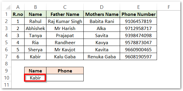
Now C10 contains our lookup_value. We want to get his phone number in cell C10. So we start typing the VLOOKUP Formula in cell C10.

=VLOOKUP(B10,

Where B10 is our lookup_value argument.

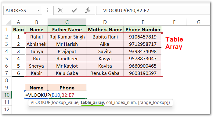
Step 2 – Specifying table_array argument of VLOOKUP Function

The next argument is table_array. Table_array contains the range of cells having all records. An important point to note here is that the function will search the lookuo_value only in the first column of the table_array.

Here the name Kabir would be looked at in the Name Column ( Column B ). So our table_array becomes B2:E7.

In this example, the table_array cannot be A2:E7. If we did so, then the first column would be R.no. We just cannot search for the name Kabir in the R.no column

So the formula in cell C10 becomes:-

=VLOOKUP(B10,B2:E7,

Step 3 – Passing the col_index_num

col_index_num is the column number from which we want our result, Here we want the phone number of Kabir. So the column containing the Phone Numbers would be the col_index_num.

The numbering of columns depends on the table_array. The first column of table_array is numbered 1.

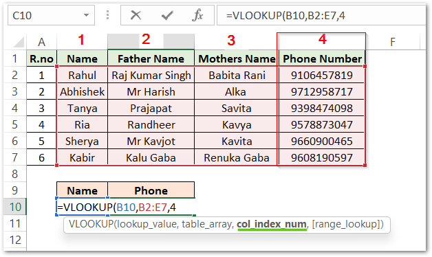
Therefore the Phone Number becomes the 4th column and the value of col_index_num is 4.

The last argument is [range_lookup]. It will be FALSE for the exact match. However, the formula becomes.

=VLOOKUP(B10,B2:E7,4,FALSE)

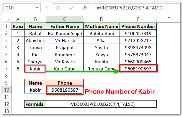
As a result, we get Kabir’s Phone Number as 9608190597.

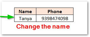
We can also change the name in cell B10 to get the phone number of another student.

If you type a name whose record is not in the list then we get a #N/A error. You can customize the error message using the IFERROR Formula.

Important Points about VLOOKUP Function

There are some important things to know about VLOOKUP Formula as follows.

• The limitation of this function is that it can only look for the values to the Right of it. i.e We can not get the R.no of a student from its Name ( R.no to its left ).
• If there are multiple records for the same lookup_value, then the value corresponding to the first match of lookup_value is considered.
• You cannot add or delete columns in between the first column and the column specified by col_index_num. The formula would not be updated because of the hard-coded column index and we will get inappropriate results.
• The col_index_num cannot be greater than the total number of columns in the table_array otherwise we get a #REF! error.

This brings us to the end of the blog.

Thank you for reading.