VLOOKUP Function with Drop Down List

In this blog, we are going to combine the functionality of the VLOOKUP Function with the Data Validation – Drop Down List feature. This is a super handy feature of the VLOOKUP Function. Let’s see how this works.

Use of LOOKUP Function

The VLOOKUP Function is used for vertical lookup. The function helps us to look for a piece of information about the lookup_value.

For example, let us suppose we have records of college students in a course.

In this value, the lookup value is in red box cell C11 which has the name “Tanya”. The formula is in the green box cell that returns the Phone Number of Tanya from the data in range A1:E7.

Whenever we type a new student’s name in cell C11, his/her phone number appears in cell D11 ( if present in the list ).

Need of a Drop Down List

In this case, there is a possibility of any spelling mistake in typing of student’s name in cell C11. Consequently, because of the incorrect spelling of the name, the VLOOKUP formula would not return the student’s phone number even if it exists on the list.

This is why we apply data validation to the VLOOKUP formula’s lookup_value.

With the use of a Drop Down list, we can replace the student name ( in cell C11 ) with a list from which we can choose the name whose phone number we want to look.

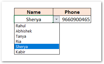
So now, you see that we have replaced the manual typing of student names ( lookup_value ) with the selection of names from the drop-down list. We can choose the name on the list from the arrow button and get his phone number in the adjacent cell.

Every time, we can simply click on the down arrow to the right of lookup_value and choose an entity from the list to get its information from all the records.

How to Combine a Drop Down list with VLOOKUP Function?

Now, we are going to implement this functionality which is divided into two main steps.

Step 1 – Writing the VLOOKUP Formula

Let us suppose we have the accounts of different persons in a bank as follows.

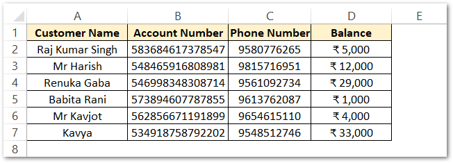
Here, we will create a lookup formula. We want to get the customer’s account balance from his name.

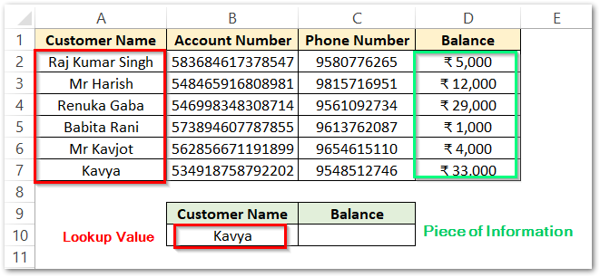
Use the following VLOOKUP Function Formula in cell C10.

=VLOOKUP(B10,A2:D7,4,0)

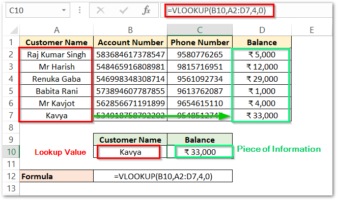
The formula returns the Balance of the Customer Name mentioned in cell B10.

Explanation – We have supplied the lookup_value argument as cell B10 as the value to search in the given data. The next argument table_array is A2:D7 which contains the data. col_index_num is the column number from which we want the result. Since Balance is the 4th column, therefor we supply 4. The last argument is 0 for the exact match.

The function looks for the name Kavya ( B10 ) in the first column ( A ) of table_array. Once the name is found, it returns its balance ( from column D )

Step 2 – Applying Data Validation to Lookup Value

The Drop Down list would add to the Lookup_value cell. Here, B10 has our lookup_value so we would attach a list to this cell that contains the name of all customers.

To make a drop-down list:-

• Select Cell B10 and go to Data Tab on the Ribbon.
• In the Data Tools Group, click on the Data Validation button.

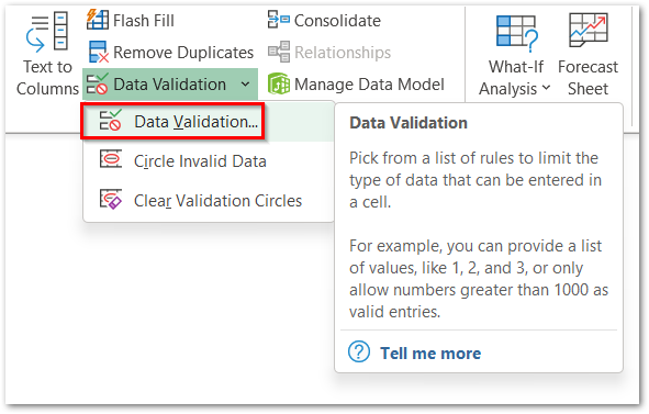
• This opens the Data Validation Dialog box. Choose the List in Allow field.
• Click on the arrow button next to Source Field. Select the range A2:A7 and press Enter key.

• Click on the OK button.

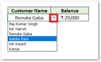
You will see a down arrow button next to cell B10.

You click on this button and choose the customer name from the created list and the VLOOKUP Function returns the balance in cell C10.

This brings us to the end of the blog.

Thank you for reading.