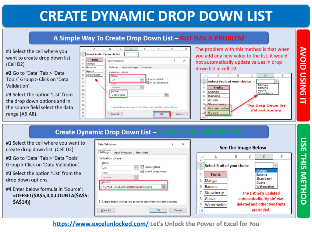
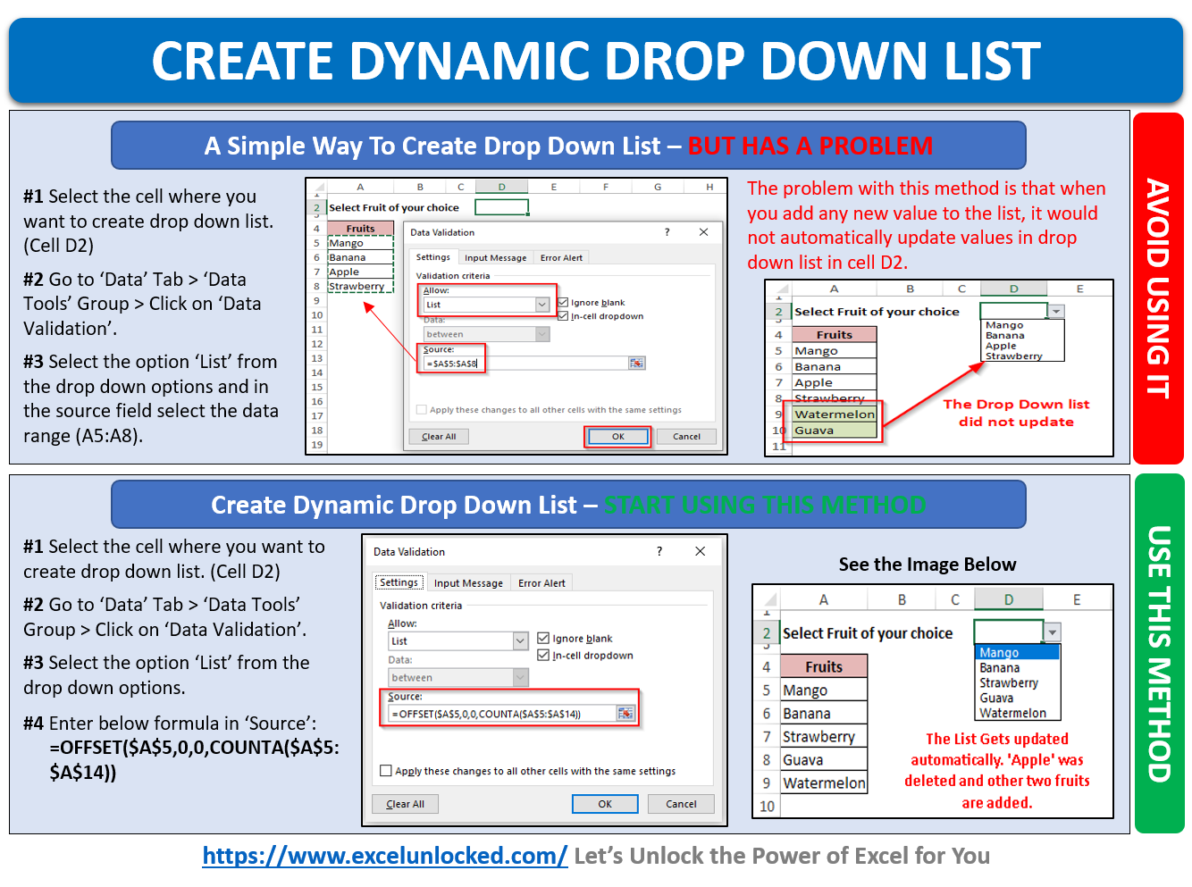
Do you know that you can even define a dynamic drop-down list in Excel? The excel data validation rule along with =OFFSET() formula would help us create a dynamic drop-down list.
When you create a drop-down list using the “Data Validation” dialog box, you specify the range of the cells which would be included in the drop-down list. However, it then remains fixed. It means, where you want to add a new element in the list, you need to manually extend the range of selected cells in the “Data Validation” dialog box.
To learn more about creating a drop-down list in excel, refer to our blog on “How to Create a Drop-Down List in Excel“.
This blog aims at unlocking the technique of creating a dynamic drop-down list that works even when new values or elements are added to the list.
Also Read: How to Create a Drop-Down List in Excel
Create Dynamic Drop Down
Follow the below steps to achieve the same :
Step 1: Enter the following data in an excel worksheet as shown in the below screenshot :
Step 2: Select the cell where you want to insert the data validation rule. In our case, we would create the drop-down list in cell D2.
Step 3: Go to the “Data” tab and click on the option “Data Validation”. It is available under the group named “Data Tool”.
The dialog box named “Data Validation” would pop on your screen.
Step 4: Select the option “List” from the drop-down menu as a validation criterion.
Step 5: In the “Source” field, enter the following formula:
=OFFSET($A$5,0,0,COUNTIF($A$5:$A$200,”<>”))
The =COUNTIF() formula would search and count for the non-blank cells within the range of cells and enter the count into the =OFFSET() formula to generate the list.
Step 5: Finally, click the “OK” to exit and activate the data validation.
With this, we have completed with this technique. Let us now test this functionality.
Firstly, click on the cell where you have entered the data validation rule (in our case it is cell D2). You would notice a down arrow symbol on the right side of the selected cell.
Click on this down arrow symbol. The list would appear in the drop-down. You would see that there are five elements (values) in it.

Now enter new element(s) or value(s) in the list as shown in the screenshot below :
Check the drop-down list in cell D2.
You would now notice that the new element(s) – Watermelon and Pineapple automatically get added to the drop-down list.
This brings us to the end of this blog.

