In this blog, we would learn how to create a drop-down list in excel. This tool is a very user-friendly tool and helps us in creating interactive excel dashboards.
Before starting with this tutorial, let us understand what exactly is the Excel drop-down list.
Excel Drop-down list is a tool that helps the user to select the values in excel cells from the predefined list.
There are multiple ways using which you can create an excel drop-down list.
- Selection of drop-down list from cells
- By entering the values manually
- Using =OFFSET() function.
Let us now start with this tutorial and try to understand each of the methods with the help of examples.
Creating Drop-Down List by Selecting a list from cells
This is the most used method to create a drop-down list in excel. Follow the below steps :
Step 1 : Enter the list as shown in the screenshot below:
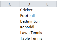
Step 2 : Select the cell where you want to insert the drop-down list.
As we want to get our list in cell B2, therefore, cell B2 is my active cell.

Step 3 : From the tabs in the excel ribbon, click on the tab “Data”. Click on the “Data Validation” button under the group ‘Data Tools’.
Consequently, the “Data Validation” dialog box would appear:

Step 4 : Under the “Validation Criteria”, select the option “Lists” from the drop-down options.
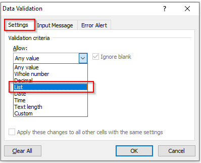
Step 5 : The “Source” field would appear.
Check the “In-cell dropdown” checkbox (as shown in the screenshot below). If it is unchecked, the drop-down list functionality will not work.
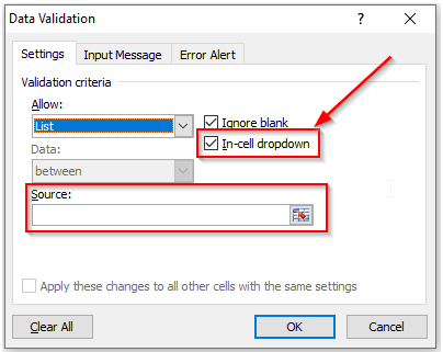
Step 6 : In the “Source” field mention the reference of range of cells (of which you want to create the drop-down the list) as below
=$D$1:$D$6
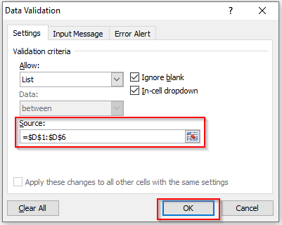
Or you can also select the range of cells. For this, click on the selection button adjacent to the “Source” field entry box, and then select the cells (list) for which you want to create the drop-down list with the help of a mouse.
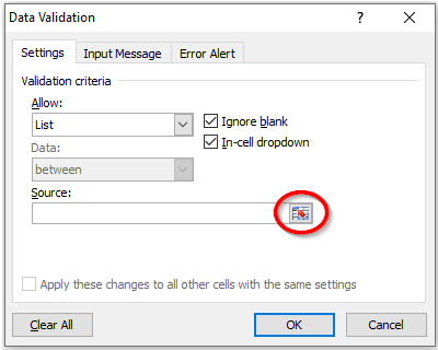
This brings us to the end of this method.
Now, it is time to test this.
Now, select cell B2. This is the cell where we have created the data validation.
As a result, you would see a downward-facing arrow on the right of the selected cell.

Click on this downward-facing arrow. You would see that your list appears as a drop-down list.
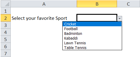
Now, Rover your mouse cursor over the list to select the value of your choice.
Consequently, you would notice that the value you chose appears in the selected cell.
Create Drop-Down List by Entering Values Manually
In the above method, we learned how to create the drop-down list by giving cell references. In this section of the blog, we would learn how to create the drop-down list manually. (without giving reference of any cell or range of cells).
Suppose you want to create a drop-down list for “True” and “False” manually without giving any cell reference. Follow the below steps:
Step 1: Click on the cell where you want the drop-down list. Therefore, I have selected cell B2.

Step 2 : From the options available under the excel ribbon, click on the tab “Data” tab. Now, select the option “Data Validation” under the group ‘Data Tools’.

As a result, you would see the “Data Validation” dialog box.
Step 3 : Under the “Validation Criteria”, select the option “Lists” from the drop-down options.

The “Source” field would appear:
Step 4 : In this field, we need to enter the values/elements for which we want to create the drop-down list separated by a comma and a space character (, )
In our example, we want to insert “True” and “False”. Therefore, write the following in the “Source” field section.
TRUE, FALSE
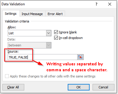
Press “Ok” button.
Finally, we have completed all the steps.
Now, to test it, follow the below procedure.
Go to cell B2. As soon as you click this cell, you would see a downward-facing arrow on the right of the selected cell.

Click on this downward-facing arrow. As a result, you would see that TRUE and FALSE appears as a list.

Rover your mouse over the drop-down list and select the value of your choice. As a result, you would notice that the value you chose appears in the cell.
Drop-Down list Using =OFFSET() function.
In addition to the above two methods, you can also create a drop-down list in an Excel cell by using =OFFSET() formula.
Follow the below steps:
Step 1 : Firstly, Click on the cell where you want to insert list.
In our example, we want to create the drop-down list in cell B2, therefore, I have selected cell B2.

Step 2 : From the Excel ribbon bar options, click on the tab “Data”. And select the option “Data Validation” under the group ‘Data Tools’.

As a result, the “Data Validation” dialog box would appear on your screen.
Step 3 : Under the “Validation Criteria”, select the option “Lists” from the drop-down options.

Step 4 : The “Source” field would appear.
Now, check the “In-cell dropdown” option. If it is unchecked, the drop-down list will not work.

Step 6 : In the “Source” field, enter the following formula :
=OFFSET(D1,0,0,6)
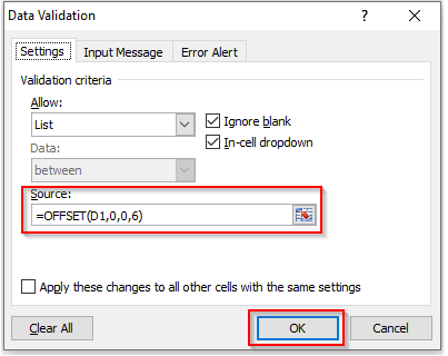
Now click on “Ok” button.
You would notice that the drop-down list is now available in the selected cell.

Explanation of the formula: The =OFFSET() formula returns the list of items from the list.
There are 3 mandatory arguments and 2 option arguments of this formula.
The first argument is the cell reference of the first value in the list. The second and third arguments are the column and the row numbers which are specified as 0 as we don’t want to offset the cell reference. The fourth attribute is the height of the list which in our case is 6 (as our list contains 6 values or elements).
This brings us to the end of this blog. Hope you have found this blog useful. Share your views and comments in the comment section below.

