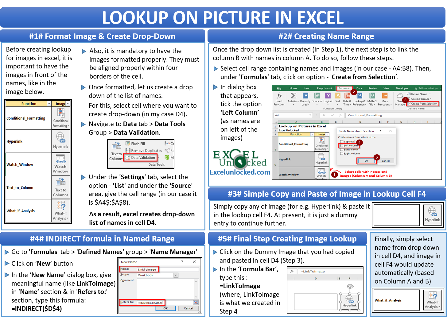
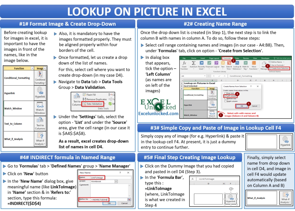
In one of our previous blog, we had unlocked the technique to insert and lock the picture into cells in Excel. So, let us move one step further. In this blog, we would learn to create a dynamic image or picture lookup such that we can lookup on the picture in excel based on the value in the cell without using any VBA code. With this, as the cell value changes, the picture placed in the adjacent cell changes.
You can apply this technique to lookup flags, company logo, products, employee pictures, and many more.
Download the sample file using the ‘Download’ button and practice along with as you go through this blog.
At the end of this blog, you would be able to do this ….

So, let us now get started with learning this technique.
Step By Step Guide – Lookup on Picture in Excel
Follow the below step by step guide on creating lookup on pictures in excel.
Step 1 – Formatting the Images and Creating Drop-Down List
Before creating lookup for images in excel, it is important to have a list of pictures against its description. Also, it is important to have the images formatted and organized inside the four borders of the cells.
By formatted image, it means, all the pictures should have the same height and width, they should be aligned properly and should be within the cell borders. You can do the formatting for all the pictures by selecting a picture and using CTRL + A keyboard shortcut to select all of them at one go.
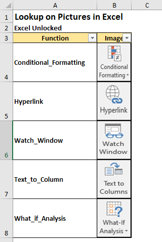
It is important to note that the names (in Column A) should be the one-word names. This is because, in the next step, we are going to create a Named Range for this list of names. The named range can only accept one word.
Now, we need to create a drop-down list for these names so that selection can be made using the drop-down arrow. To do this, select the cell D4 and go the ‘Data‘ ribbon tab > ‘Data Tools‘ group > ‘Data Validation‘ option.

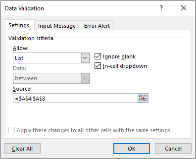
Under the ‘Settings’ tab, select the option – ‘List’ and under the ‘Source’ area, give the cell range (in our case it is $A4$:$A$8). Refer to the image below.
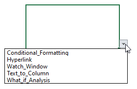
As a result, you would notice that the excel creates drop-down list of names in cell D4-
Step 2 – Creating Name Range for Images
Once our list is ready, the next step is to create a named range by linking the names in column A with the images in column B. This is the reason, why the images in column B must be within the four borders of the cell.
To assign the name to the picture cell (column B), follow the below steps.
Firstly, select the cell range containing names and the images (in our case – A4:B8). Then, under the ‘Formulas‘ tab, click on the option that says – ‘Create from Selection‘ (Defined Names Group).
Also Read: Assign Macro to Image and CheckBox
In the small dialog box that appear, select the checkbox ‘Left column‘ (as the names are on the left of the images).
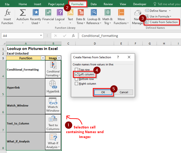
Once this is done, click on any of the cells containing pictures (column B) and check the ‘Name box’ (left-side of the Formula bar). You would see the name of the cell is the name of the adjacent cell in Column A.
Step 3 – Copying and Pasting Image in Destination Cell
Simply copy any of the images (let’s suppose, Hyperlink) and paste it in the lookup cell F4. You can choose the image of your choice. This image is not yet fixed. We would create it a dynamic according to the list once all steps are completed. At present, it is just a dummy entry to continue further.
Step 4 – INDIRECT Formula in Named Range
The next step is to create a named range with INDIRECT function in excel. The INDIRECT function helps in creating a cell address or cell reference by entering a text inside the INDIRECT function.
For creating lookup on the picture in Excel, the INDIRECT function would create a cell reference of column B, using the text in cell D4.
Go to ‘Formulas‘ ribbon tab > ‘Defined Names‘ group > ‘Name Manager‘ option.

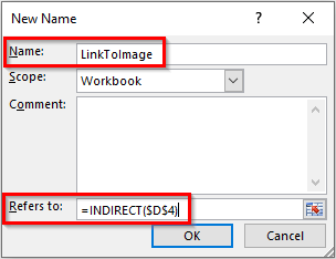
In the dialog box that appears, click on ‘New‘ button. The ‘New Name‘ dialog box would appear on your screen wherein give a meaningful name (like – LinkToImage) in the ‘Name‘ section. In the ‘Refers to:‘ section, type the formula =INDIRECT($D$4), and click OK, as shown in the image below.
Then Close the Name Manager.
If you are not fond of using the INDIRECT function, you can even use the INDEX and MATCH function, like the way explained by Sumit Bansal.
Step 5 – Final Step is to Create LOOKUP on the Picture
Finally, we have now all the required settings in place to create lookup on the picture in Excel. Follow the below steps:
Select the dummy image that you have just copied and pasted in cell F4 (Step 3). Now, in the formula bar, write the following, and press Enter.
=LinkToImage
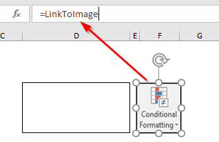
=LinkToImage is the nothing but the recent Name created in the Name Manager (Step 4).
Explanation On Working of This Technique
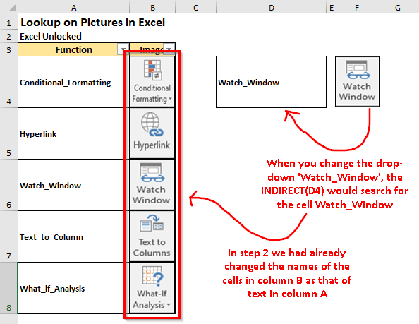
In Step 5, the dummy image in cell F4 has been given a name as =LinkToImage. In the ‘Name Manager’ we have created a named range =LinkToImage which refers to the value in cell $D$4.
Also in step 2, we had given a same name to the image cells (column B) as that of the names (column A).
So, when you change the drop-down value in cell D4, the =INDIRECT($D$4) function in the name manager searches for the cell reference with the name as D4. The excel would find the cell reference with the name in cell D4 in column B (where cells B4, B5, B6, and so on are the names in column A), as defined in step 2.
With this, we have reached the end of this blog. Share your views and comments in the comment section below.

