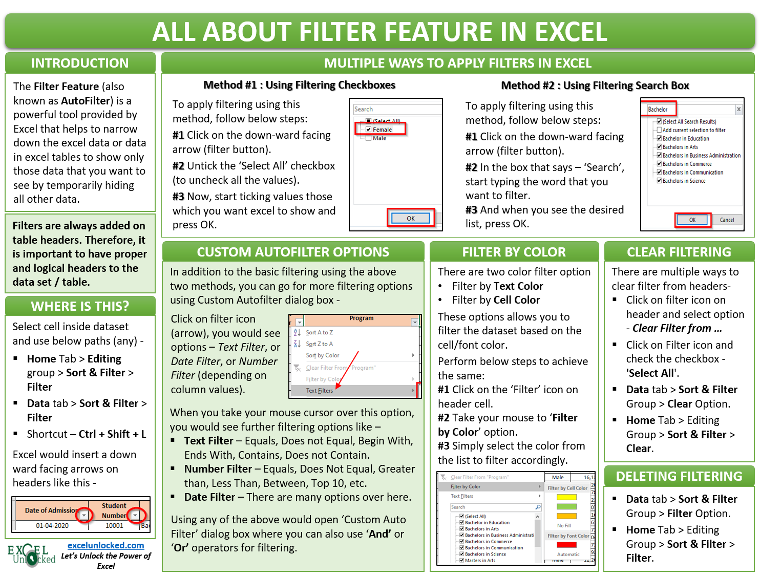
The Excel Filter Feature is a great tool that proves to be a lifesaver at the time when you are working with huge data in Excel. In this blog, we would unlock this filter feature in Excel. We would learn how to filter huge data in excel. We would also get into answering the following common questions – how to filter values, or numbers, or dates and time in Excel, how to use filter using wildcard characters in excel, how to filter using the search box, how to filter by text or cell color.
Sample Data – Download Sample File
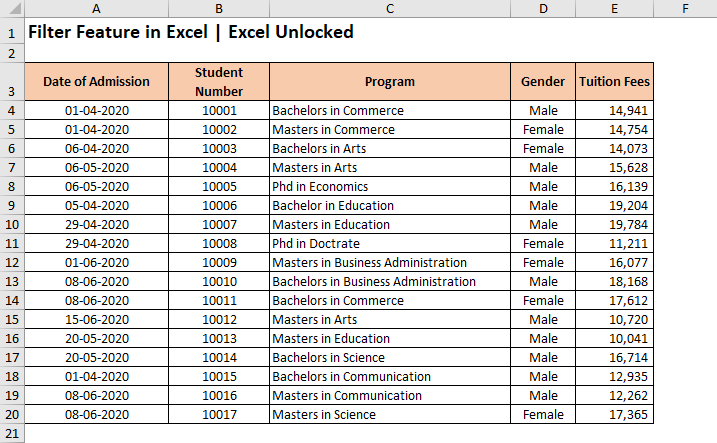
In this blog, we would be using the below data. Kindly download and practice along with using the Download button.
- Sample Data – Download Sample File
- What is the Purpose of Filter Feature in Excel?
- Adding Filter Option on Header Rows
- Simple Ways to Filter Your Data Set in Excel
- Filter Data Using Filter Search Box in Excel
- Clearing Filter on Columns in Excel
- How to Filter Values or Text in Excel?
- How to Filter Numbers in Excel?
- How to Filter Dates in Excel?
- How to Filter By Color in Excel?
- A Solution To – AutoFilter Does Not Work After Changing Data
- Copy and Paste only Filtered Data in Excel
- Removing Filter From Headers in Excel
What is the Purpose of Filter Feature in Excel?
The Filter Feature (also known as AutoFilter) is a powerful tool provided by Excel that narrows down the excel data or data in excel tables to show only those data that you want to see by temporarily hiding all other data. In our sample data, for example, we can use this feature to condense the data such that it only shows the programs taken up by the ‘Female‘ applicants.
In a similar way, you can filter by dates, or values or by any other such criteria.
Adding Filter Option on Header Rows
The filters are always added to the headers of the data set. Therefore, it is important that your excel data must contain a header row, with logical headings. In our example, row 3 is the header row with headings describing the column data.

Once your dataset has proper headers, you are now good to insert the AutoFilter on these headers. To add AutoFilter on the header row, click on any of the cells inside the excel data set (like C7) and use any of the below-mentioned ways:
- Go to ‘Home‘ tab > ‘Editing‘ Group > ‘Sort & Filter‘ Option > ‘Filter‘ button.
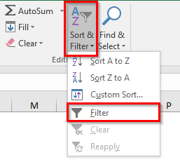
- Go to ‘Data‘ tab > ‘Sort & Filter‘ group > ‘Filter‘ Button.

- Keyboard Shortcut Method : Ctrl + Shift + L
As soon as you use any of the above methods, the excel would automatically detect the header row inside the table or data set and insert filter buttons on each of the header cells. These are the downward-facing arrows, like the way shown below:

Simple Ways to Filter Your Data Set in Excel
Once the filter option added to the headers, you are good to start filtering your data set.
With this feature, you can filter your data by a single column or by multiple columns.
Applying Filter on Single Column
To apply the filter on a single column, simply click on the filter button (downward-facing arrow) of the respective column. (Let us firstly apply the filter on the column ‘Program Name’). As a result, you would notice that all the checkboxes are checked by default.
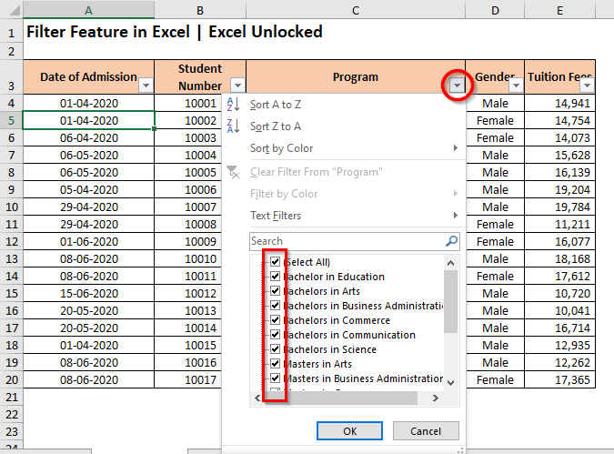
Uncheck the checkbox that says ‘Select All‘. This would remove the check boxes from all the values.
Now, start ticking the values that you wish to view and click on ‘OK’, like the way demonstrated in the below image.
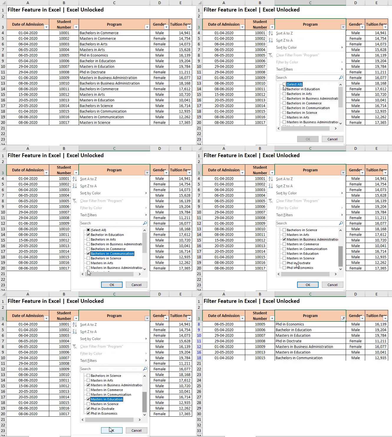
Consequently, the excel would view or show only the selected values in the column, rest all are hidden. Don’t worry excel has not deleted them, they are still there in the backend.
Applying Filter on Multiple Columns
In a similar way, you can apply the filter on other columns in the Excel Data Table. There is no limitation on how many columns to which you can apply the filter.
Let us now apply another filter on the column having header – ‘Gender‘.
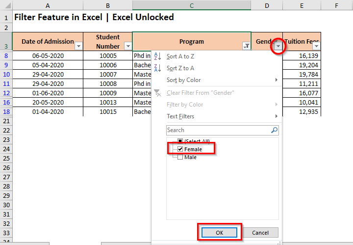
As a result, the excel would now only display the data set rows for selected ‘Program’ and for ‘Female’ candidates. All others are temporarily hidden (not removed).

Some Useful Points and Tips
Once a filter is applied on the header row-
- The Downward-facing arrow on the filtered column changes its icon which denotes that there is a filter applied to this column.
- When you take your mouse cursor over the filter button, it shows the filter values.

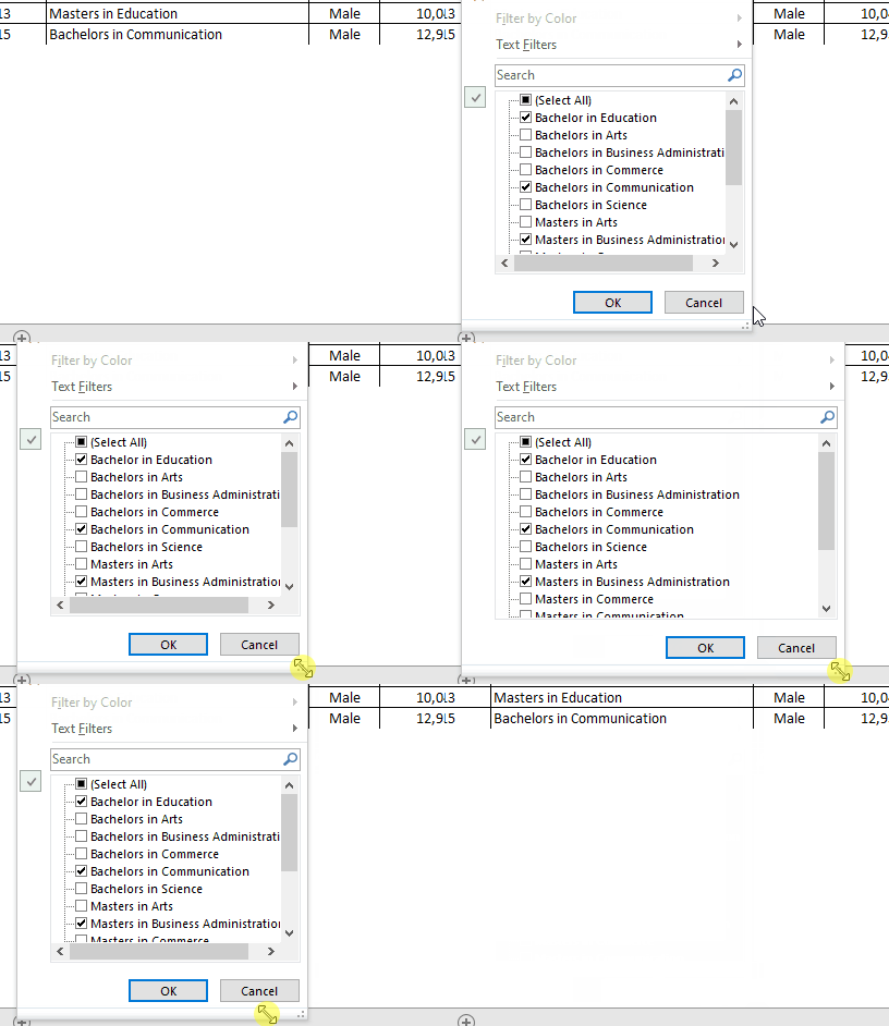
- To increase or decrease the width of the filter window, take your mouse cursor on the bottom-right corner of the filter window. Once the mouse cursor changes to a two-side facing arrow, click and drag right (to increase) or left (to decrease). See the below demonstration for more clarity.
Filter Data Using Filter Search Box in Excel
In the earlier section, we learned about how to filter your data set by selecting the checkboxes in the Filter window. There is yet another way to filter out a specific text or value or numbers or dates/time in Excel which is by using the ‘Filter’ search box. The Filter search box is placed just above the list of values in the Filter window.
To filter your data set using the ‘Filter’ search box, simply click on the ‘Filter’ drop-down icon on the header and type the search value in the search box. As a result, the excel would narrow down the list to show only the specified values. Finally, click on the ‘OK’ button to apply the filter.
To illustrate with an example, let us filter out the ‘Program’ column with the Bachelor’s degree.
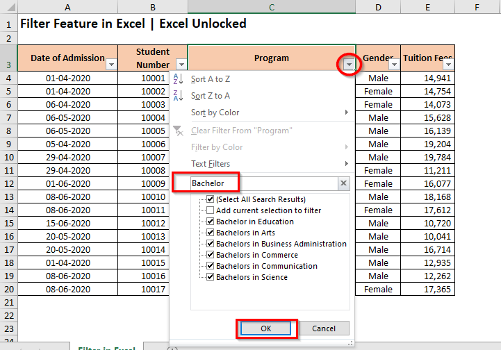
Not sure about the exact text to search, then use wildcard characters in the search box for a non-exact filter search in Excel. If you are unaware of what are wildcard characters in Excel and its usage, then please click here.
Clearing Filter on Columns in Excel
When you want to clear filter from selected or all the header columns in Excel, you can use any of the below-mentioned ways:
- Click on the ‘Filter‘ icon on the header of the column header, and click on the option that says – Clear Filter from <Column Header Name>

- Another way is to click on the ‘Filter‘ icon of the header, and check the checkbox – ‘Select All‘.
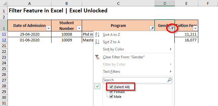
When you clear the filter from the column ‘Gender’, the data set would now only have a filter on the column header ‘Program’. It has only cleared filter from the row ‘Gender’ and has not touched any other filters.
To clear multiple filter from all the headers cells, use any of the following way:
- Click on any of the cells in the dataset and navigate to the path – Data tab > Sort & Filter Group and there click on the option that says – Clear.

- Or you can even use this – Home Tab > Editing Group. Click the option Sort & Filter > Clear.
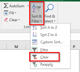
It is important to note that the above method only clears the filter from the header cell. It does not remove the filter icon from the header row. To learn how to remove the filter in Excel, wait until the end of this blog.
How to Filter Values or Text in Excel?
When you are working with text filters, there are many other text filter options available in addition to what we learned above. Below is the list of the same.
- You can filter the values or text which exactly Equals or which Does Not Equal to some text.
- Additionally, you can even filter for a non-exact match by using the Contains and Does Not Contain a text
- Or, you can even filter the values or text that starts or Begins With or Ends With a particular text.
These advanced filter options are available under the ‘Text Filter’ section of the Filter Window as shown in the image below:
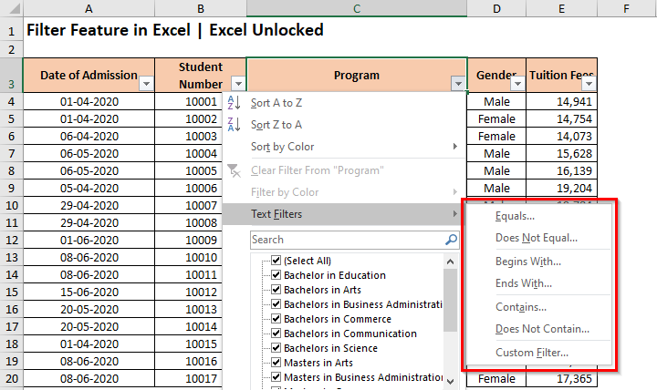
Let us understand this with the help of a small example: Let us, for example, get the program that contains the word ‘Business’ in it. To achieve it,
Click on the ‘Filter‘ icon on the column header – ‘Program’, and take your mouse cursor to the option – Text Filters.
In the list of options that come up, select the option that says – ‘Contains‘. As a result, the ‘Custom AutoFilter‘ dialog box would appear on your screen. In the input box besides the word ‘Contains’, write the text that you want to filter (in our case ‘Business’) and press OK.
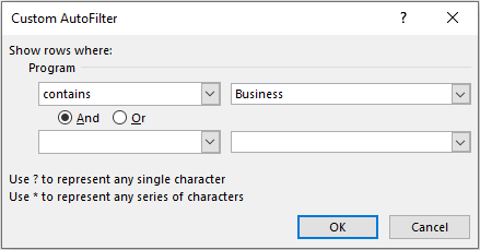
As soon as you press OK, excel would show all the values or text that contains the word ‘Business’ and will hide all other data rows.
Note that, just like Filter search box, this ‘Custom AutoFilter’ dialog box also accepts wildcard character search.
Filter Values based on Two Criteria
The Custom AutoFilter dialog box also allows us to filter out the data rows based on two criteria. Use the And and Or operator radio buttons based on how you wish to filter.
For example: Let us filter out all the programs for Commerce and Science. In this case, as we want both the values, we shall use Or operator, like this-
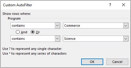
This would filter out those values which either contain the word ‘Commerce‘ or contain the word ‘Science‘.
How to Filter Numbers in Excel?
Similar to the text filter learned above, there are many additional filter options available carry Number Filters in Excel. Below is the list of the same:
- You can filter the exact number or amount by using Equals and Does Not Equal option under the ‘Number Filter’.
- Similarly, the Number Filter – Greater Than and Less Than allows us to get all values that are more or less than a specific value.
- Greater Than or Equal To and Less Than or Equal To works in a similar way.
- Between Number Filter allows you to filter out the values lies between two values (lower and upper values both inclusive)
- Other options are – Top 10, Above Average, Below Average
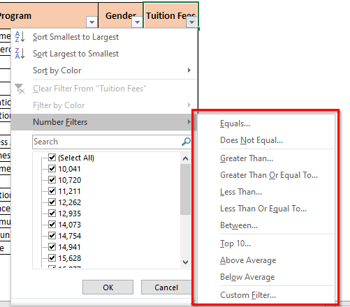
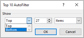
The filter option Top 10 does not exactly only mean Top 10 values. You can change it to any other value like Top 15, or Top 27 Values, and even Bottom 5 values and so on.
How to Filter Dates in Excel?
Unlike the Text and Number Filter, the Dates Filters option allows us with more advanced filtering options. The below image in itself is self-explanatory.
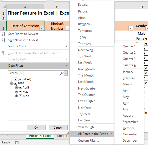
In a nutshell, below options are available for filtering dates in Excel –
- You can filter the dates which fall in the current month/week/quarter/year and even for previous and upcoming (i.e. next) month/week/quarter/year.
- Additionally, you can filter out by an exact date, or date that falls before or after a particular date, or between two dates.
- Excel provides with an option to filter all the dates in a particular month or quarter (regardless of the year in which it falls)
- You can create a custom date filter using the ‘Custom AutoFilter’ dialog box to which you are already aware of using.
Important to notice – Excel by default groups all the dates by year, months, and then the days. You can expand or collapse the groups (year, months, and days) to filter the dates and check/uncheck it to filter accordingly.
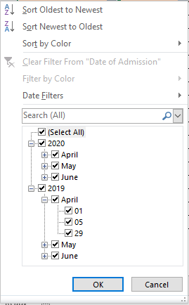
In the above image, you can see that all the dates are grouped by years first (2020 and 2019). Within the years there are months and then the days in the month. If you clear the checkbox for 2020, then the excel would only show the dates that lie in 2019.
How to Filter By Color in Excel?
When the data set contains any text with color or any cell with a background color, you can use the ‘Filter by Color‘ option in the ‘Filter’ Window to filter the dataset by a specific text or cell background color.
Let me explain this with a small example. I am changing the background color of different cells to yellow, orange, and green. Also, I have the font color in a few of the cells as ‘Red’.
To filter the values based on color, simply click on the ‘Filter’ drop-down arrow button on the header cell and take your mouse cursor over the option that says – ‘Filter by Color’.
As a result, you would see that excel lists all the cell and font color. You can choose the color that you want to filter with.

Let us, for example, filter the programs by Red font color. The result of the filter would be as below.

Quick Way to Filter By A Specific Cell’s Value, Font Color, Cell Color or Icon
Instead of using the ‘Filter’ drop-down icon to filter, you can even filter the dataset based on a specific cell’s value, icon, or font and cell color. To do so, follow the undermentioned steps:
- Right-click on the cell that contains the color by which you want to filter. Let us, in this case, filter by yellow color. Therefore, I have right-clicked on C4 (as it has a yellow cell color).
- Take your mouse cursor to the option that says – ‘Filter‘, and click on the option – ‘Filter by Selected Cell’s Color‘.
As a result, excel would filter the dataset based on the cell color – Yellow, as demonstrated in the below image:

A Solution To – AutoFilter Does Not Work After Changing Data
When you make any changes in the filtered data, you would notice that excel does not refresh the filter automatically. Yes, that is absolutely true. You need to reapply the filter in order to refresh the data and apply the filter on the changed data. There are a couple of ways to do the same, as listed below:
- Using Filter Window – After making changes in the filtered data, simply click on the ‘Filter’ drop-down arrow on the header cell and click ‘OK’ in there. However, there is are exceptions to this method. This would not work when you apply ‘filter by color’ or ‘Number Filter/Text Filter/Date Filter’. This technique only applies when you use the search box to filter out the data.
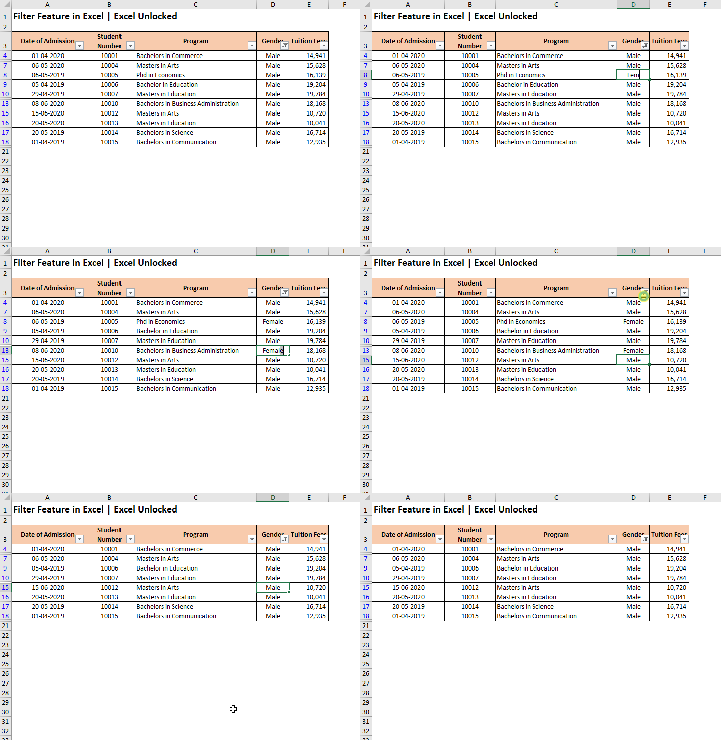
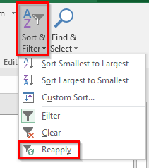
- Using Reapply Option – After making changes in the filtered data, simply navigate to the Data tab > Sort & Filter Group > Reapply Option. The keyboard shortcut key for the same is Ctrl + Alt + L.

This option is also available in the Home Tab > Editing Group > Sort & Filter Option > Reapply.
Copy and Paste only Filtered Data in Excel
There are two possibilities to copy and paste only filtered data in Excel.
Copy and Paste Filtered Data Including Header Row
Simply, click on any of the cell in the filtered area, and press Ctrl + A to select the entire excel table or data set. As a result, you would notice that excel selects the entire table including both data rows as well as the header row. Now, press Ctrl + C to copy the selection and use Ctrl + V at the destination location to paste the filtered data cells.
Copy and Paste Filtered Data Excluding Header Row
To copy and paste only filtered data (without header row), select the top-left cell of the data (which in our case it is C4). Press keyboard keys Ctrl + Shift + Down_Arrow and then press Ctrl + Shift + Right_Arrow (instead you can even use Ctrl + Shift + End). Any of these ways would select the entire data set (excluding headers). Now, use Ctrl + C to copy the selection and then Ctrl + V to paste the filtered data set at the destination cell.
Usually, when you copy the filtered dataset using the above methods, excel does not include the hidden rows in the copy area. The hidden rows are excluded and it only takes the visible rows while copying. However, sometimes when your data is huge, it may not work in expected behavior. In those cases, to play safe, you can use the GoTo (F5) > Special > Visible Cells Only feature to select only the visible rows. The keyboard shortcut for the same is Alt + ; (semi-colon).
Removing Filter From Headers in Excel
Finally, let us now learn how to remove filters from the excel header row. There are multiple ways using which you can remove filters, as listed below-
- The easiest way is to use the keyboard shortcut – Ctrl + Shift + L.
- Another way is to use ribbon path – Data Tab > Sort & Filter Group > Filter option OR Home Tab > Editing Group > Sort & Filter Option > Filter Option.

