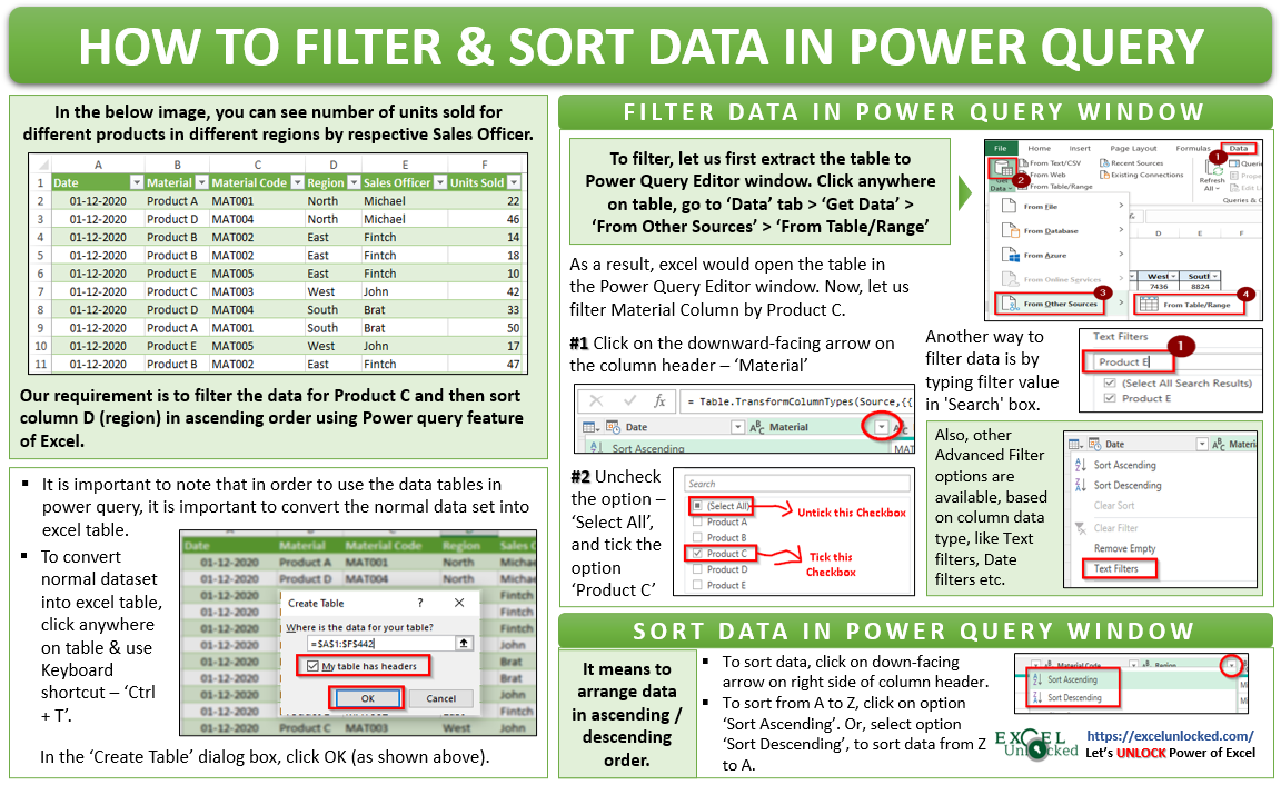
The Microsoft Excel Power Query feature is an amazing feature pre-provided by Microsoft in Excel 2016 and the later versions. I call this feature – “A Life Saver Feature” when it comes to the extraction of data from external sources into excel. The Power Query feature of Excel allows you to extract data from sources like the same workbook or another excel workbook, PDF, JSON, CSV, Text, Websites, etc. Once extracted, you can perform many types of transformation or data cleansing activities on this extracted data. One of the transformations is “Filter and Sort data in Excel Power Query”. In this blog, we would unlock the technique of how the filtering and sorting of an excel data work in Excel Power Query.
To learn about the basics of the excel power query feature and its advantages, it is recommended to go through the ExcelUnlocked Power Query overview blog. Click here to read it.
Sample Data For Filtering and Sorting
In the below image, you can see number of units sold for different products in different regions by respective Sales Officer.
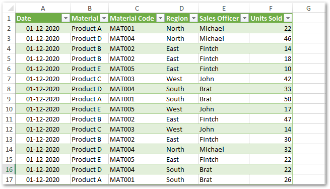
Now, we want to filter and/or sort data using Power query feature of Excel. Let us unlock this technique in the below section :). Before you go ahead with this technique, download the sample excel file and practice as you read. Click on the Download button below.
Also Read: How to Sort a Table or Data in Excel
Filter and Sort Data in Power Query [Step by Step Guide]
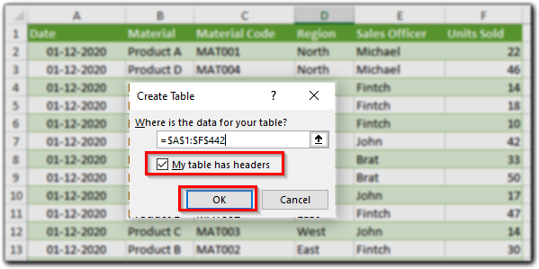
To use the Power Query feature on tabular datasets in excel (as shown in the above sample image), it is important to convert the normal tabular dataset into proper excel table.
To convert a normal table into proper excel table, simply select any of the cells within this normal table, use ‘Ctrl + T’ keyboard shortcut and click OK (in ‘Create Table’ Dialog Box). See the image below.
Once your dataset it in excel table format, we can now start with-
- Importing the Excel Table to Power Query Editor Window
- Filtering the imported data, and then finally,
- Sorting this data
Import Excel Table to Power Query Editor Window
To import this excel table to power query editor window, click any of the cells on this table. Then, navigate to ‘Data’ > ‘Get & Transform Data’ > ‘Get Data’ > ‘From Other Sources’ > ‘From Table/Range’.
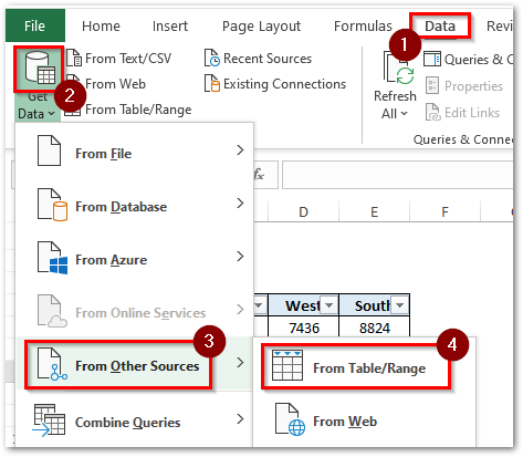
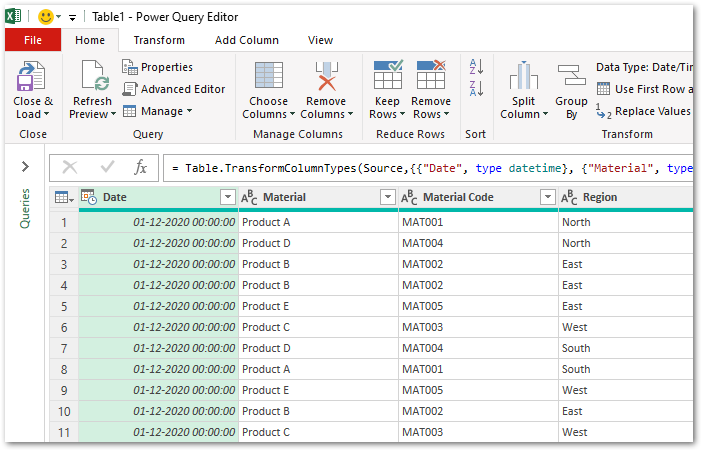
As a result, this table would get open in a new window named ‘Power Query Editor’. Also, you can see that Excel automatically detected and changed the data types of the table headers.
Filter Data in Excel Power Query Editor Window
The filter feature in power query is similar to and works just like a normal excel filter feature.
By fitering data in excel, it means to display or hide only a particular type of data in the table. For example, using this feature you can only display the sales data for Product C, and hide the others.
This option is available on the power query table column headers itself. Simply click on the downward-facing arrow on the right side of the column header to open the available filtering options, as shown below:
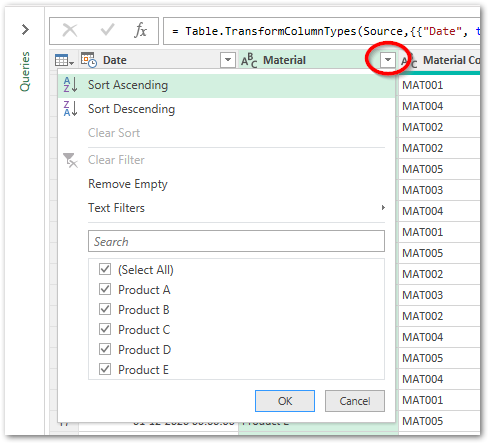
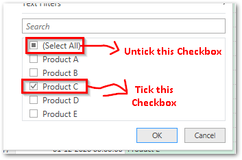
To display sales data for only Product C, uncheck the ‘Select All’ option, then select the option ‘Product C’ and click OK.
As a result, power query editor window would filter out and show the data for Product C (hiding all other Product data).
You can select show more than one value (like show both Product C and Product A), by ticking the checkbox for both the values.
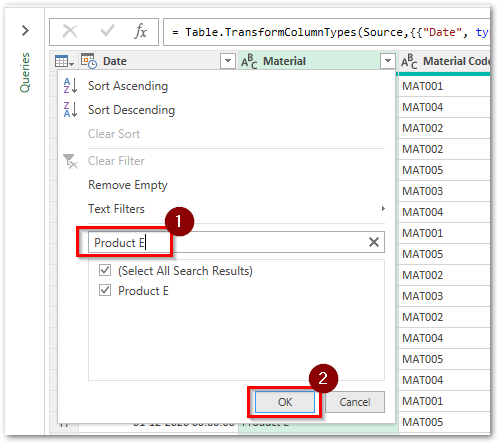
Another way to filter data is by typing the filter value or text in the Filter ‘Search’ box. See the image below.
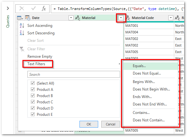
Additionally, there are some advanced filter options available based on the data type of the column header.
If you are filtering the column containing text, then you have many other advanced filtering options available. You can filter by exact text (equal to), or text that begins with or ends with a particular string, and many more.
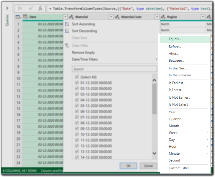
Similarly, if you apply a filter on the column that contains the date/time, then the advanced filter options change accordingly. See the image below:

Sort Data in Excel Power Query Editor Window
Sorting Data in Power Query allows you to arrange the table data into ascending or descending order.
The easiest and the most popular method to sort the column in excel power query editor window is to use the option from the filter drop down menu.
On the right side of the column header, you would find a downward-facing arrow (as highlighted below).
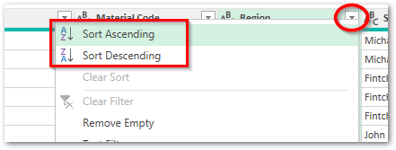
The sorting options are available in this drop-down arrow options.
To sort from A to Z, click on the option ‘Sort Ascending’. In contrast, select option ‘Sort Descending’, to sort the data from Z to A.
This option is also available on the Power Query Editor window ribbon – Home tab > Sort group. Simply, select the column and click on the AZ or ZA options to sort it in ascending or descending order, respectively.

I have, for illustration purpose, applied filter on Product C and sorted the column named Region in ascending order.
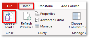
Now, let us load the this new transformed data from power query editor window to excel worksheet. To load it to excel, go to ‘Home’ tab > Close & Load’ as shown in the image below:
Finally, you have the filtered and sorted data in a new excel worksheet and excel stores this new data as queries and connection.

What Happened In Background?
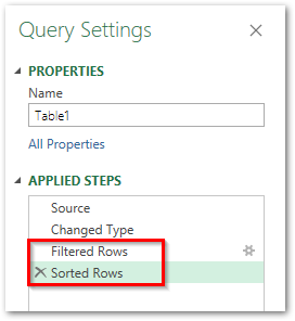
While you were doing transformations on the extracted data, the excel power query editor window was recording and storing these steps for future use.
If you notice the Query Settings pane in the ‘Power Query Editor’ window, there you can find these recorded steps.
But why did the power query editor window record the steps for you? Just for fun? No 😛
Answer to the above question -> Suppose, sometime in the future, your source data table updates with new rows of data. At that time, you can reuse these recorded steps and get the latest transformed data instantly. No need of performing the filtering and sorting steps learned above again.
Simply, right-click on the new table and use the option ‘Refresh’, to get the latest data from the source.
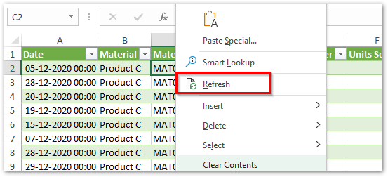
On right-click refresh, excel would extract data from source table, detect & change column header data types, apply filter on Product C and then sort the Region column in ascending order.
This is the reason, why I call the Excel Power Query Feature as a Life Saver Tool. Now, I think, you would agree with this. Right? 🙂

