How to Add Conditional Column in Excel Power Query

Excel Power Query feature is an amazing tool provided by Microsoft in Excel to get the data from various sources and transform it according to our requirements. Conditional Column is one of the transformations that you can do with the Power Query. In this blog, we would learn how to use and work with the conditional columns in excel power query.

If you are working with the Power Query feature of Excel for the first time, I would recommend you to go through our overview and basic blog. Check this link.

What are Conditional Columns in Power Query?

As the name suggests, conditional columns are the table column(s) that derive their value based on the value in another column within the table.

Let us understand this by taking a sample example. The below sample data shows the number of units sold by different sales officers in a particular month.

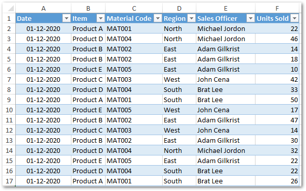
Now, suppose we want to show the commission payable for each of the records in a new column, based on the below logic.

• If the number of units sold is more than or equals 30 units then, the column should show the text as ‘Eligible for commission @ 10%’.
• If the number of units sold is more than 10 units but less than or equal to 30 units, then ‘Eligible for commission @ 5%’.
• The new column should show the text as ‘No commission’ when units sold are less than or equal to 10 units.

Power query conditional column feature will help you to achieve this instantly.

Adding Conditional Column in Excel Power Query

All the transformation tools and options in Power Query are available in a separate ‘Power Query Editor’ window.

Therefore, working with power query transformations involve two steps:

1. Extracting the data from the source table into the Power Query Editor window.
2. Applying the conditional column feature in this new window.

Below is the detailed explanation on above two steps.

Import the Table into Editor Window

The power query feature does not understand normal excel dataset tables. In order to work tabular dataset in power query, it is must to have an excel understandable table format.

To convert the normal dataset into excel table format, select the table range and then press shortcut keys Ctrl + T. This would open up a new dialog box. Finally, click the option OK to make an excel table.

The power query import options are available in the ‘Data’ tab of Excel ribbon options under the ‘Get & transform Data’ group.

Now, click anywhere on the excel table and go to ‘Data’ > ‘Get & Transform Data’ group > ‘Get Data’ > ‘From Other Sources’ > ‘From Table/Range’.

Consequently, this would instantly display the excel data table in power query editor window.

Applying Conditional Column in Power Query Editor Window

To add the condition-based column, the power query editor window uses the ‘Add Conditional Column’ dialog box. You can find this under the ‘Add Column’ tab > ‘Conditional Column’ option.

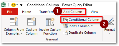
As a result, the ‘Add Conditional Column’ dialog box would appear on your screen.

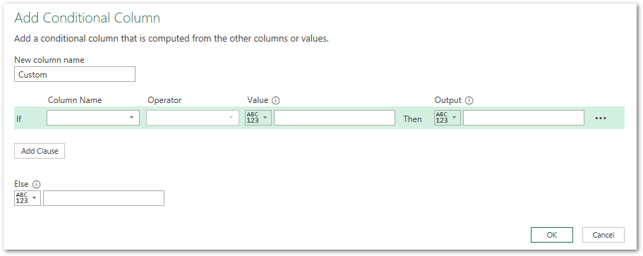
Give a name to the new column in the ‘New Column Name’ input box (eg ‘Commission Payable’).

The next part is the IF condition part and the expected output if the condition is fulfilled.

• Column Name section represents the column to check for the condition.
• Operator section enables you to select the operator (equal to, less than, etc.) for the condition.
• Value section is used to provide a value to be checked for condition fulfillment.
• Output input box is used to specify the expected output if the above condition is satisfied.

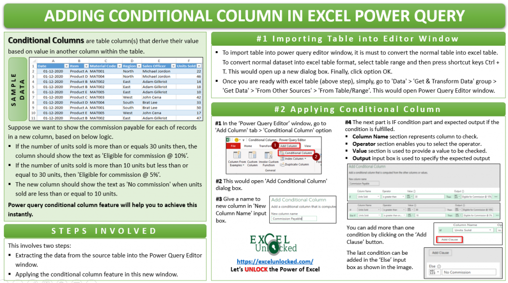
Let us make the settings for our three conditions.

Condition 1:- If the number of units sold is more than 30 units then, the column should show the text as ‘Eligible for commission @ 10%’.

Now click on the ‘Add Clause’ button to add the second condition.

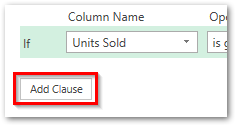
Condition 2:- If the number of units sold is more than 10 units but less than or equal to 30 units, then ‘Eligible for commission @ 5%.

Condition 3:- Text ‘No commission’ when units sold are less than or equal to 10 units.

Mention the output in the ‘Else’ input box.

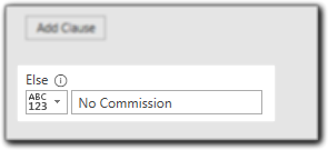
As soon as you click on the OK button, you would return back to the power query editor window.

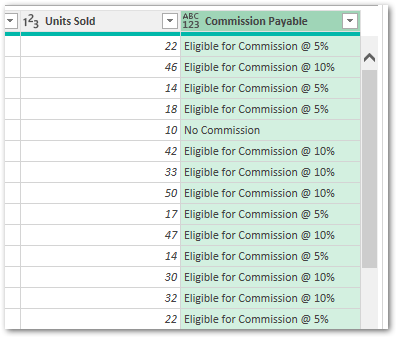
Consequently, you would notice that the power query window adds a new column – ‘Commission Payable’, at the right end of the table.

How to Export Data from Power Query Editor To Excel

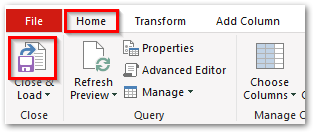
To get the table with a conditional column back to the excel worksheet, navigate to the ‘Home’ tab (in the Power Query Editor window) > ‘Close & Load’ option, as shown below.

That’s It, You finally have your table with the conditional column back to excel. Wasn’t it so easy !! 😎