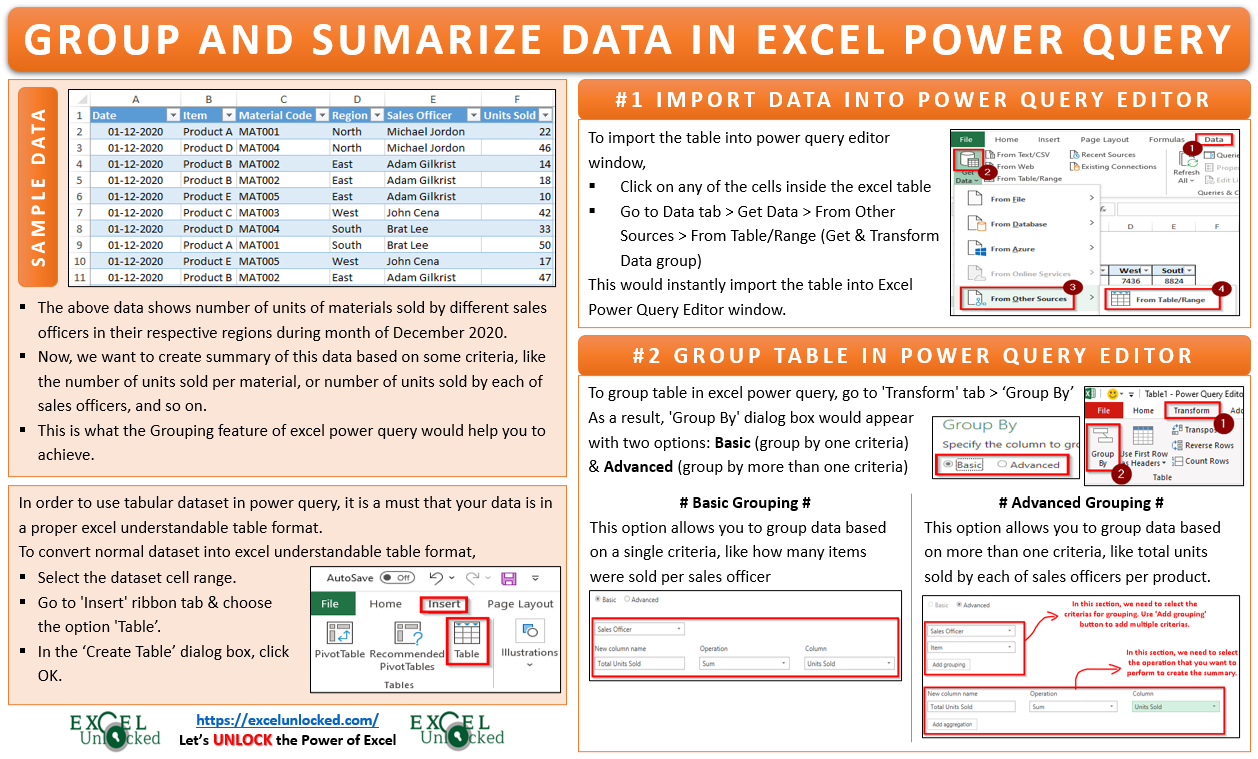
The Excel Power Query tool is like a lifesaver tool when you want to extract some of the data from external files and folders or from internal excel tables and place it into an excel worksheet. However, the utility of this feature is not just to import data from the external files and folders, but you can use the Power Query excel feature to transform this imported data. One of the transformations that you can do in power query is the grouping and summarizing of data in Excel. In this blog, we would unlock this technique on how to group and summarize excel table data using the power query feature.
What is Grouping and Summarization of Data in Excel?
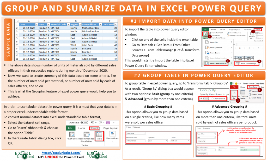
Suppose you are working with a huge set of sales data in excel for a company. See an extract of the data in the image below:
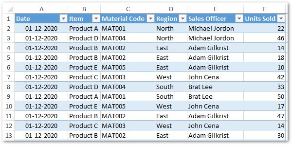
The above data shows the number of units of materials sold by different sales officers in their respective regions during the month of December 2020.
Now, we want to create a summary of the data based on some criteria, like the number of units sold per material, or the number of units sold by each of the sales officers, and so on.
This is what the Grouping feature of excel power query would help you to achieve.
Steps to Group Data in Excel Using Power Query
In order to work with the excel data in power query, the first step is to import this data into the ‘Power Query Editor’ window. The Power Query Editor window is a separate window in Excel which has all the tools used to transform and clean the data.
To import excel data into the power query editor window, it is a must that your data is in a proper excel understandable table format. By proper excel table format, it means the table format that excel has defined.
You can convert the normal table to make it an excel understandable table, follow these steps:
- Select the entire dataset range of cells (i.e. your table area).
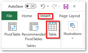
- Go to the ‘Insert’ ribbon tab, and click on the option ‘Table’.
- The ‘Create Table’ dialog box would pop out on your screen. Simply click ‘OK’ to activate it.
1# Import Excel Table Into Power Query Editor
Now, once the excel table format is ready, let us now import it into the power query editor window.
- Click on any of the cells inside the excel table.
- Go to Data tab > Get Data > From Other Sources > From Table/Range (Get & Transform Data group)
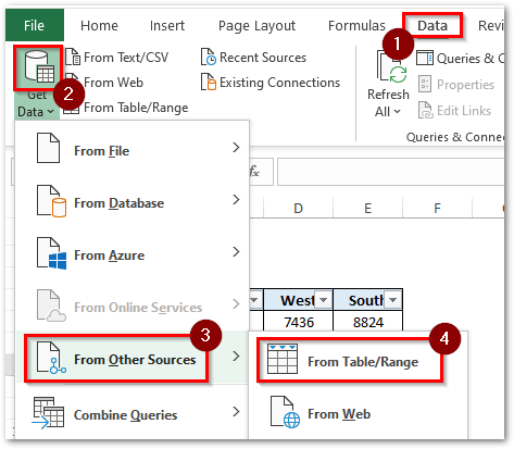
This would instantly import the table into Excel Power Query Editor window.
Now, let us move to step number 2 and learn how to group this imported table.
2# Group Table in Excel Power Query Editor Window
- Go to the ‘Transform’ tab in the Power Query Editor window and you will find the option called ‘Group By’. Click on this ‘Group By’ button.
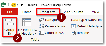
- As a result, the
- Here, you can either perform a ‘Basic’ grouping or an ‘Advanced’ grouping of data.

Let us learn both these grouping options in the coming sections.
Basic Grouping in Power Query – Group Data in Excel By Single Criteria
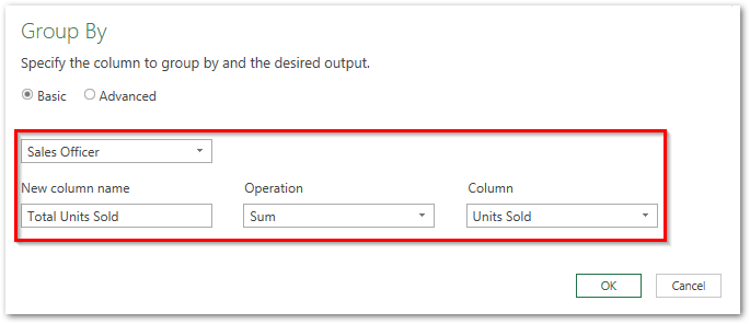
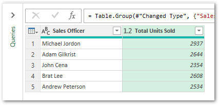
The ‘Basic’ grouping allows you to summarize data table based on a single or only one criteria. For example, we can group our data set to find how many items were sold per sales officer. Follow the below steps:
- Firstly, select the radio button ‘Basic’ in the ‘Group By’ dialog box.
- Then, click on the drop-down button to select the column header name based on which you want to group the data. In our example, it is ‘Sales Officer’.
- Then, in the ‘New Column Name’ input box, give a name to the new column, as ‘Total Units Sold’. And, select the operation as ‘Sum’. In the last drop-down list, select the column name from the drop-down on which you want to perform the operation, viz. ‘Units Sold’.
As soon as you click on ‘OK’, you would notice that the power query creates a new summary table based on the stated criteria.
Also Read: Custom Columns in Table in Excel Power Query
Advanced Grouping in Power Query – Group Data in Excel By Multiple Criteria
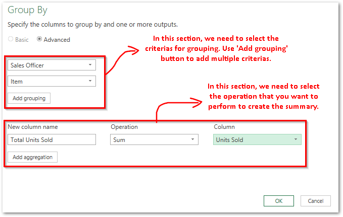
The ‘Advanced’ grouping allows you to summarize data table based on multiple criterias. For example, let us find total units sold by each of the sales officers per product.
- Firstly, select the radio button ‘Advanced’ in the ‘Group By’ dialog box.
- In the first drop-down list, select the first criteria, like ‘Sales Officer’. To add the second criteria, click on button ‘Add grouping’ and select the second criteria like ‘Item’.
- Finally, similar to Basic grouping, give a name to the new column, as ‘Total Units Sold’. Select the operation that you want to perform on the new column, for example, ‘Sum’ and select the column on which you want to perform the operation, ‘Units Sold’.
See the image below:
As soon as you click on the ‘OK’ button, you would notice that excel groups and creates a summary for you based on the multiple criterias specified.
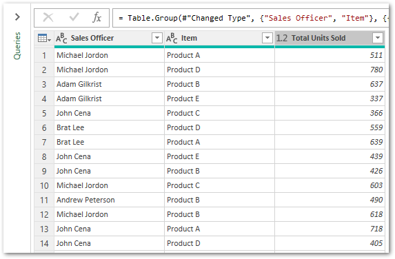
After performing the above grouping transformation, you would notice that the power query editor window has stored this step in the ‘Applied Step’ section.
Get Power Query Data to Excel
Finally, let us take this summary from power query editor window back into excel worksheet, using below steps:
Click on the ‘Home’ tab (in the power query editor window) and choose the option ‘Close & Load’. See the image below:

This would instantly move the data from power query window to excel. That’s it, so simple and easy to use feature of Excel !! 😉
Readers of this post are also interested to learn ExcelUnlocked Free Pivot Table Course.

