I am sure that every Excel user has some or the other day heard about an amazing Excel feature – Pivot Table. A Pivot Table is a powerful reporting feature used for summarizing a huge dataset in Excel.
In this first tutorial of Free Excelunlocked Pivot Table Course we would get into some basics and overview stuffs on Pivot Table for beginners. In the upcoming sequential blogs, we would dig a bit deeper and explore other Advanced Pivot Table features in Excel.
So let us begin now. Happy learning this amazing and powerful Excel tool.
Pivot Table in Excel – Meaning and Purpose
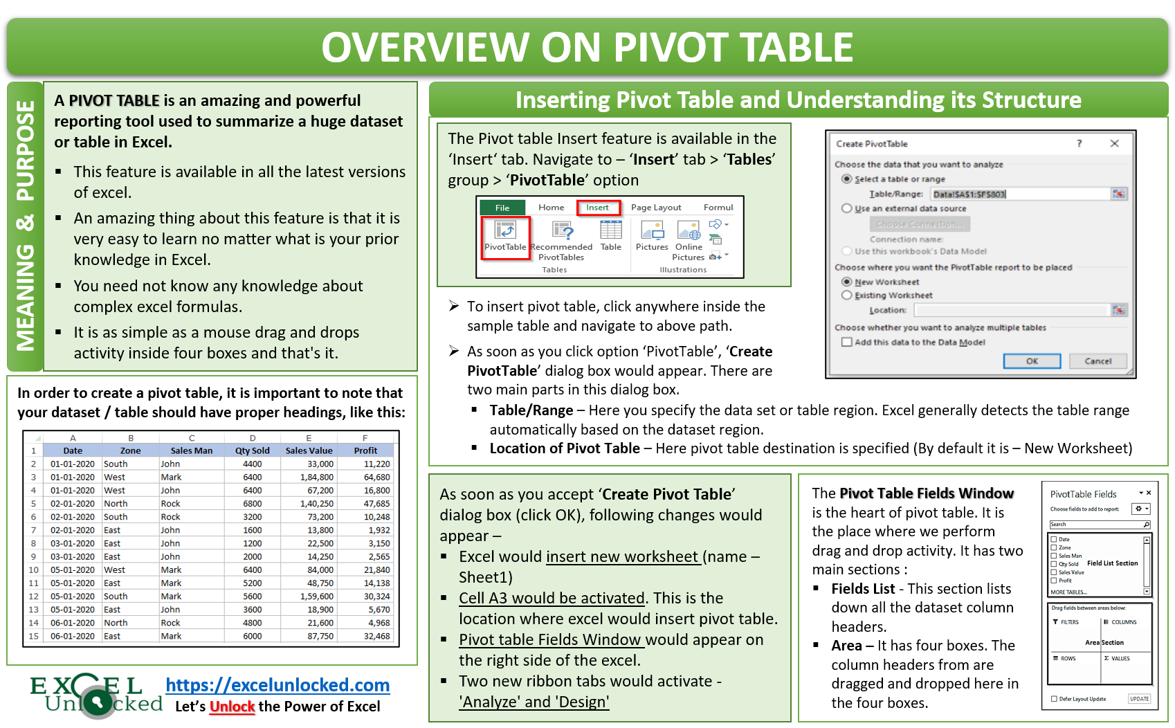
A Pivot Table is an amazing and powerful reporting tool used to summarize a huge dataset or table in Excel. This feature is available in all the latest versions of excel.
When you have a huge data set and you want to create a summary of it to portray it to your manager, the pivot table tool is a great helper.
An amazing thing about this feature is that it is very easy to learn no matter what is your prior knowledge in Excel. You need not know any complex formula to learn this feature.
It is as simple as a mouse drag and drops activity inside four boxes and that’s it. Your reports are ready then within a few drags and drops.
In order to create Pivot table, it is important that the dataset or table should have proper column headings.
Sample Data
The below image shows the sales made in the year 2020 by different salesmen in four regions (zones) showing quantity sold, sales value, and profit earned.

The sample dataset image above is just a few lines out of 1000s of rows of data. Click on the Download button below to download the entire sample dataset and practice as you read.
From Where To Insert Pivot Table in Excel
The Pivot Table Feature is available under the ‘Insert‘ tab in the ribbon options. Click anywhere inside the excel dataset, and then navigate to the ‘Insert‘ tab > ‘Tables‘ Group > ‘Pivot Table‘ option, as shown in the image below.

As soon as you click on the ‘Pivot Table‘ option (highlighted above), a new dialog box would appear with the title – ‘Create Pivot Table‘. See the image below.

In the ‘Create PivotTable‘ dialog box, there are two main sections-
- Table/Range – In here, you need to specify the data set or table region. Excel generally detects the table range automatically. As you can see, in our case excel detected the entire table range (Data!$A$1:$F$803).
- Location of Pivot Table – Here you need to specify the location where you want excel to create the pivot table. By default and also recommended to let excel create the pivot table in ‘New worksheet’. If you want to have it in the current worksheet, select the checkbox ‘Existing Worksheet’, and specify the location cell reference in the ‘Location’ input box.

Generally, the default settings work in most of the cases where excel create the pivot table in a new worksheet. Let us in this case, go with the default options itself by clicking on the ‘OK’ button.
As soon as you click OK, following changes would appear on your excel window-
- Excel would insert a new worksheet with a default name (Sheet1).
- In the new worksheet, cell A3 will be active. This is the location where the pivot table report will be created.
- Pivot Table Fields window will appear on the right of the excel window.
- Two new ribbon tabs – ‘Analyze‘ and ‘Design‘ would appear and activate.

Understanding PivotTable Fields Window
The PivotTable Fields window is said to be the heart of the Pivot Table creation. It is the place where we actually do the drag and drop activity based on which the Pivot table gets created.
Let us explore this window. There are mainly two sections in this window:
- Fields List Section – This section lists down all the dataset column headers.
- Area Section – The Area section contains the four boxes which are Filters, Columns, Rows, and Values. The column headers from the fields section are dragged and dropped here in the four boxes. According to where you drop the fields, excel generates the pivot table.

With this, you have completed the first milestone of the Pivot Table Course. In the next blog, we would go through some real-life examples on how to use the Pivot Table feature to create summarized reports.
Check out other Excel Pivot table related blogs on Free Pivot Table Course by Excelunlocked.