In our previous tutorial on the Free ExcelUnlocked Pivot table course, we had learned how to group dates in the pivot tables. In continuation of the same, let us now learn how to group numbers in the pivot table in excel.
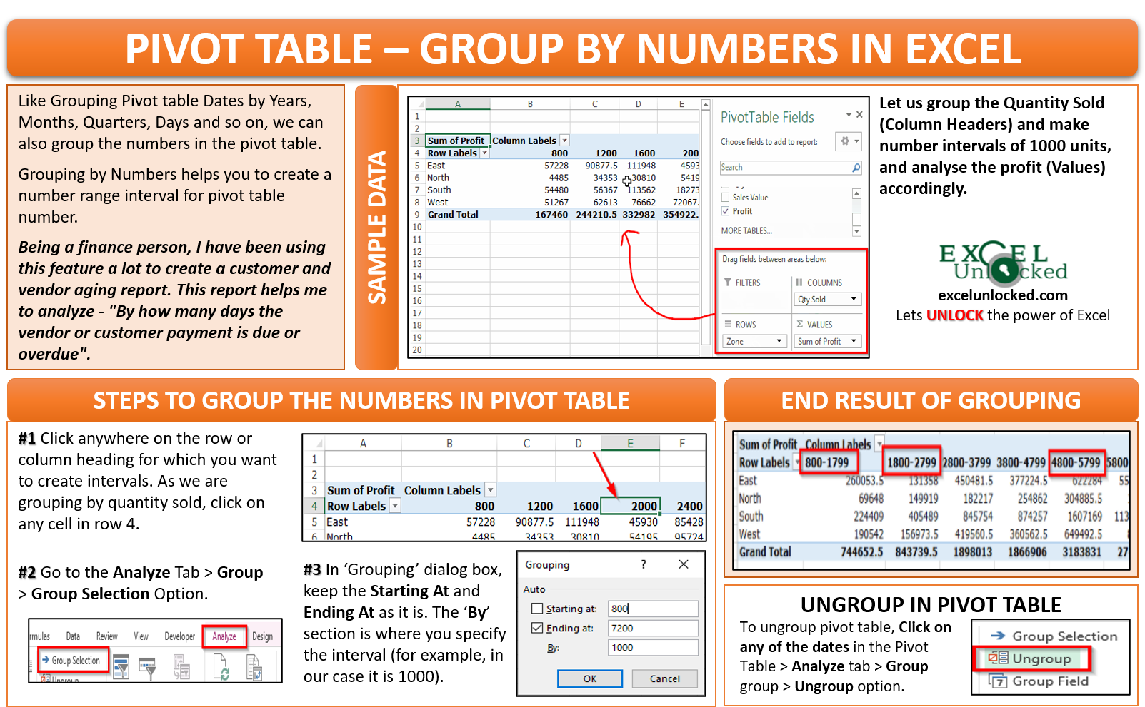
Being a finance person, I have been using this feature a lot to create a customer and vendor aging report. This report helps me to analyze – “By how many days the vendor or customer payment is due or overdue“.
So, let us now learn to create a pivot table with a number range interval using the group by numbers feature of excel pivot table.
Before, you start learning this feature, download the sample file. Click on the download button below and practice as you read.
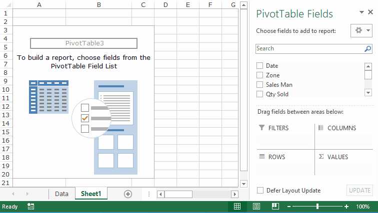
Creating a Sample Pivot Table
Based on the sample data, let us first create a report which shows the total profit earned (zone-wise) and then create the intervals for quantity sold (at every 1000 units).
To create a pivot table (already learned in this tutorial) follow below steps –
- Click anywhere on sample dataset or table and then navigate to Insert tab > Tables Group > Pivot table option. And click on the ‘OK‘ button in the ‘Create PivotTable‘ dialog box.
- In the ‘PivotTable Fields‘ window, drag and drop the ‘Zone’ field under ‘Rows’ area, ‘Quantity Sold’ field in the ‘Columns’ area, and ‘Profit’ in the ‘Values’ area.
Let us now start grouping the numbers in Pivot table in Excel.
Group Numbers in Pivot table in Excel
Follow the undermentioned steps for grouping numbers in pivot table in Excel-
Group Numbers in Pivot Table in Excel
- Number Row/Column Selection :
Click anywhere on the row or column heading for which you want to create intervals. In our case, it is ‘Quantity Sold’ which is to be grouped. Therefore, I have selected cell E4 (alternatively, you may select any cell in row 4).

- Navigation to Group Selection Path :
Go to the Analyze Tab > Group group > Group Selection Option. As a result, a new dialog box appears with the title – ‘Grouping‘.

- Understanding ‘Grouping’ Dialog Box
In the ‘Grouping‘ dialog box, by default, the Starting At and the Ending At number would be auto-populated as the minimum and maximum number in the range. Keep it is as it is (800 and 7200).
Similarly, the ‘By‘ input box is where you need to specify the intervals (i.e. number of items in each group). As we want to create a group/range of 1000 values, specify the By value as 1000 and click OK.


Finally, as a result, excel would group the pivot table number and make a batch of 1000s, like this –


How to Ungroup in Pivot Table Excel?
To ungroup the pivot table numbers, the path is simple.
Simply, click on the grouped numbers (intervals) in the Pivot Table > Analyze tab > Group group > Ungroup option.

Finally, you have completed the fifth milestone of the ExcelUnlocked Pivot Table Course.
Check out other Excel Pivot table related blogs on Free Pivot Table Course by Excelunlocked.