Grouping the Data items in the pivot table help us quickly reach conclusions without going into a deep study. We can define ranges for numbers, Quarters, or Months for Dates and Manually Group the text values to make groups of data in the pivot table and read them combined.
Let us see how we can achieve it!
Grouping Dates (Data) by Months and Quarters in Pivot Table
We have learned to make a Pivot Table in Excel in our previous blog.
So in this example, let us say we have the orders summary placed on different days of a month as follows:-
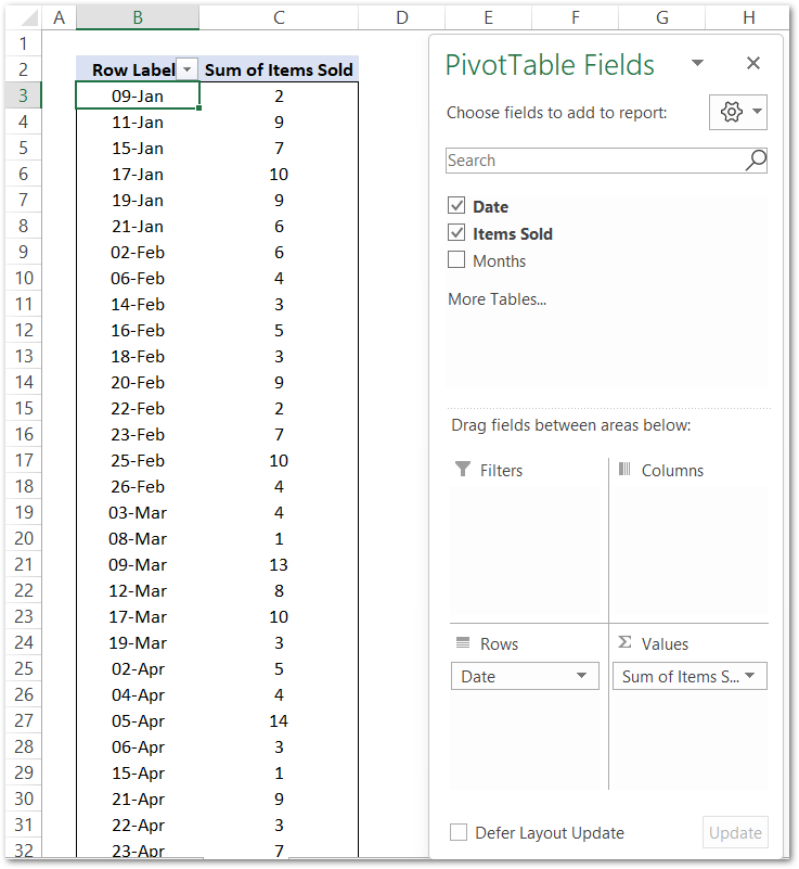
We have got the Dates and then the number of items sold on that date of the year. It is easy to read the items sold on each date but what if I want to check up on the total sales for January?
The answer is simple. We can just group the dates ( data) into months in the pivot table. To group the dates:-
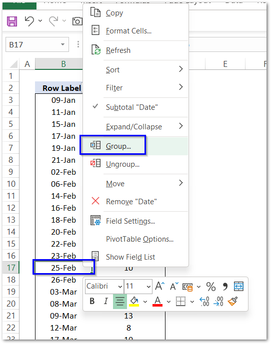
- Right-click on any one of the dates in the pivot table.
- Choose the option Group from the shortcut menu.
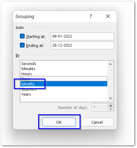
- Mark the Option for Months in the Grouping Dialog Box and click Ok.
This gives us the pivot table as follows:-
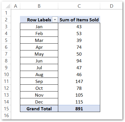
And from the pivot table, we come to know that the total sales were maximum in the month of September (147) and minimum in March (39).
We can even do nested grouping. In other words, groups combined to make some more groups.
What if we group these months (group of dates) into Quarters (group of months). All we need to do is, select both months and quarters in step 3.
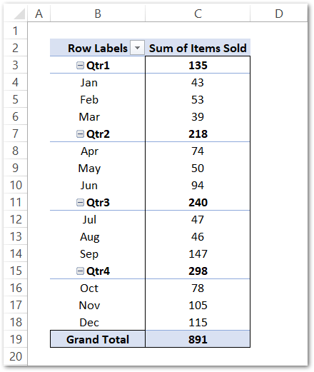
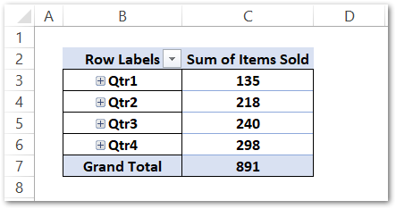
You can press the minus button before the Quarter names to hide the contents and this can be toggled.

Grouping the Weights into Ranges
Let us say we have generated a pivot table that has the weights and the corresponding number of class students with that weight.
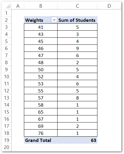
Now we have got the number of students corresponding to the value of the weight but we would now form ranges for these weights. To do so:-
- Right-click on any weight value and choose the option Group.
- Set the starting (41) and ending (80) along with the dividing factor (10)
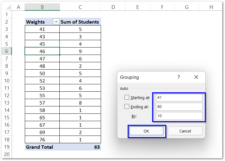
This forms the ranges with a width of 10 kgs that start from 41 kgs and end at 80 kgs as follows:-
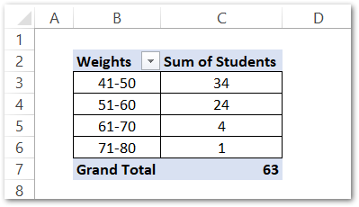
So you can see most of the students have their weights between 41-50 kgs.
Grouping the Texts
Let us say we have the sales of different vegetables and fruits of a shop as follows:-
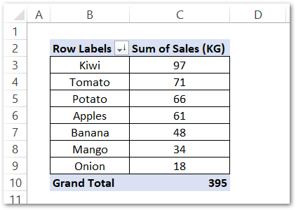
Now we want to make two groups of vegetables and fruits each. To do so:-
- Hold the Ctrl key and choose Kiwi, Apples, Banana and Mango.
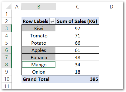
- Right, CLick and then choose the option for Group.
- Group1 will be formed, rename it to Fruits from the formula bar.
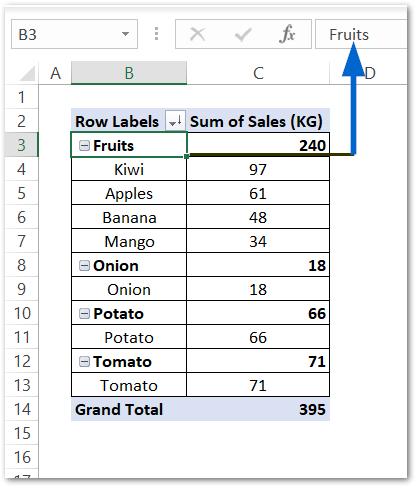
- Select the remaining items i.e onion, potato, and tomato.
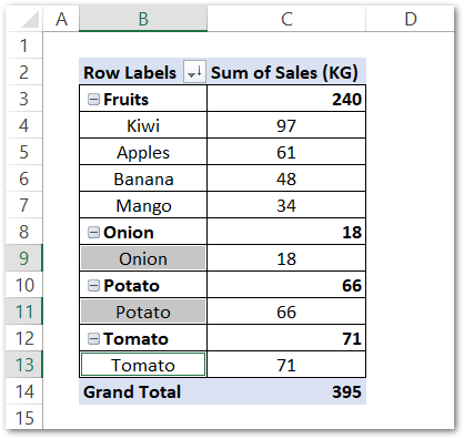
- Group them from the shortcut menu and rename group2 as vegetables.
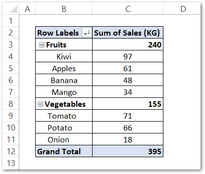
We hope that you have learned how to Group Data in Pivot Tables.
This brings us to the end of the blog.
Thank you for reading.

