In this blog, we would learn how to group and ungroup the rows in excel to organize our data table properly. This technique would allow you to collapse and expand the rows that contain similar content. It is very easy to group and ungroup the rows in excel because it does not require the formation of any complex formulas.
This technique will work when the data table is structured without any blank rows and column headings.
In this blog, we would unlock the technique to group and ungroup the rows manually as well as automatically.
Let us now begin with this excellent data structuring functionality.
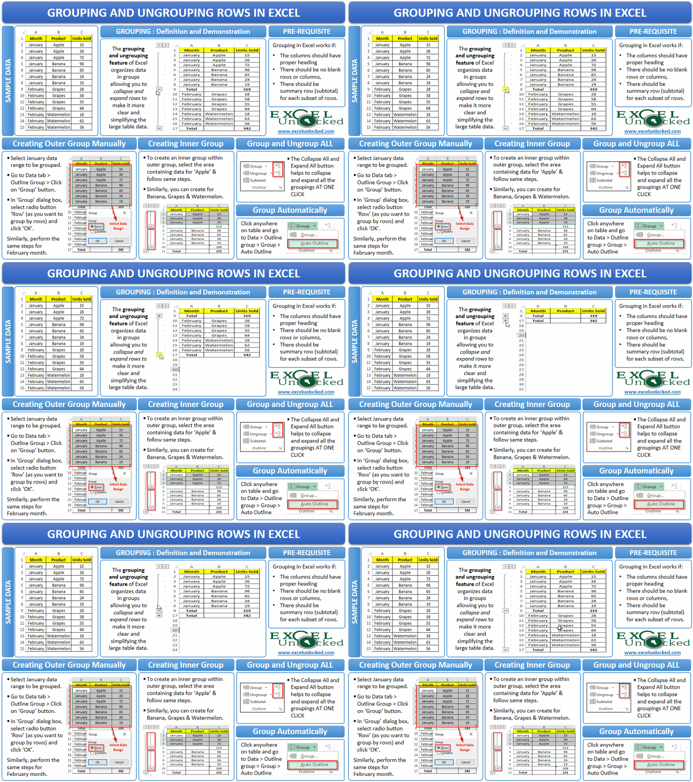
Group the Rows Manually in Excel
Creating the Outer Group Manually
To group the rows manually follow the below steps steps
Step 1: Select the data that you want to group into one group. In this case, we are only grouping January month’s sale.
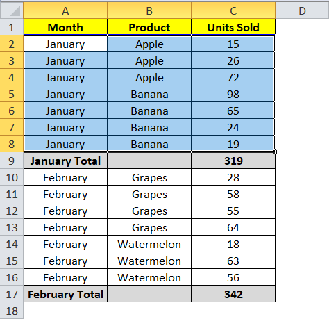
Make sure that you are not selecting the headers of the columns.
Step 2: Under the ribbon options, click on the tab “Data”. On the extreme right of the ribbon option, you would find a button “Group” (under the group ‘Outline’)

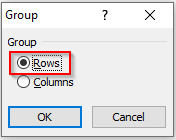
The group dialog box would open. In this dialog box, select the option “Rows” and click the “OK” button.
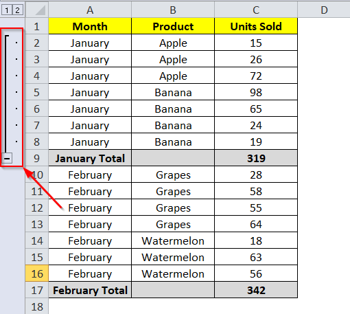
On the left side of the worksheet, you would notice a minus button (-). This is the collapse button. Click on this button to collapse the group.
Also Read: Group and Ungroup Worksheets in Excel
As soon as you click on the collapse button, you would notice that the selected cells got collapsed and you now have the plus like symbol (+) on the left side of the workbook.
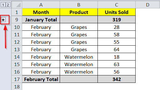
This is the Expand button. On clicking on this expand button, January sales data is visible.
Similarly, you can create more outer groups. For example, you can create the groups for February.
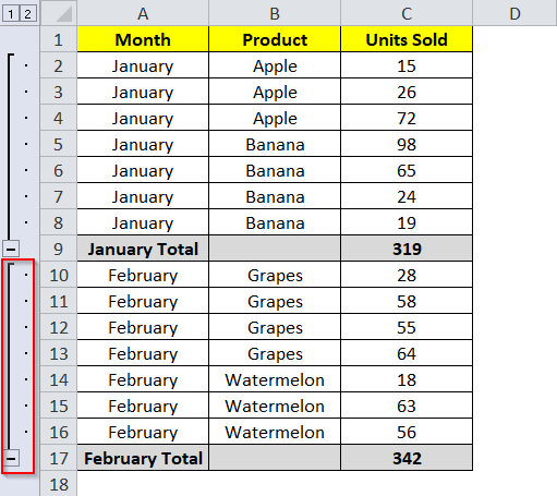
To collapse and expand the data, you can either click on the minus and plus like symbols on the left side of the worksheet, or you can use the “Show Details” and “Hide Details” options on the ribbon as shown in the screenshot below :

Creating the Inner Group manually
Suppose within the group “January” we want to create subgroups (called as an inner group) for Apple and Banana and in “February” for Grapes and Watermelon.
To create the inner rows within the outer rows, follow the below steps :
Step 1: Select the rows for which you want to create the inner group.
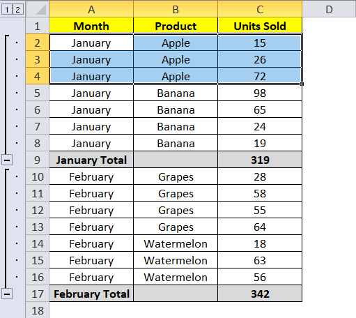
Step 2: Under the ribbon options, click on the tab “Data”. On the extreme right of the ribbon option, you would find a button “Group” (under the group ‘Outline’)

The group dialog box would open. In this dialog box, select the option “Rows” and click the “OK” button.

You would now notice that your worksheet has an inner group as shown in the screenshot below :
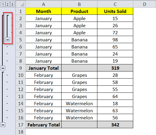
Similarly, you can create inner groups for Banana, Grapes, and Watermelon.
Group the Rows Automatically
If your dataset just contains one level of the information, then, in that case, you can automatically create the groups without manually selecting the rows.
Follow the below procedure to automatically group the rows in excel.
Step 1: Select any of the cells in the dataset.
Step 2: Under the ribbon options, click on the tab “Data”. On the extreme right of the ribbon option, you would find a button “Group”, click on that and select the option “Auto Outline”.

Finally, you would notice that the data gets organized in groups with an outline bar on the left side of the worksheet as shown in the screenshot below :
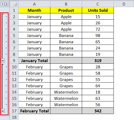
Now,
What if your data subtotal rows are above the data as shown in the screenshot below.
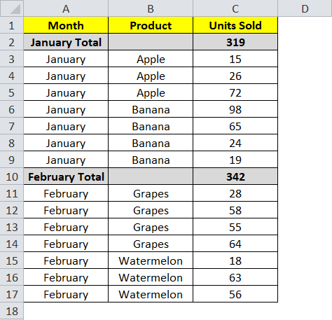
In that case, you need to change the direction of the group by following the below steps :
Step 1: Go to the “Data” tab. Under the “Outline” tab, click on the “Direction” dialog box launcher. It is a small square button with an arrow inside it on the bottom right of this group.

Step 2: In the “Direction” dialog box, uncheck the “Summary rows below details” option as shown in the below screenshot.
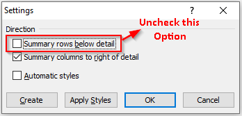
After changing the direction of grouping, you can now start the grouping of the dataset (either manually or automatically)
After grouping, your dataset would look like this :
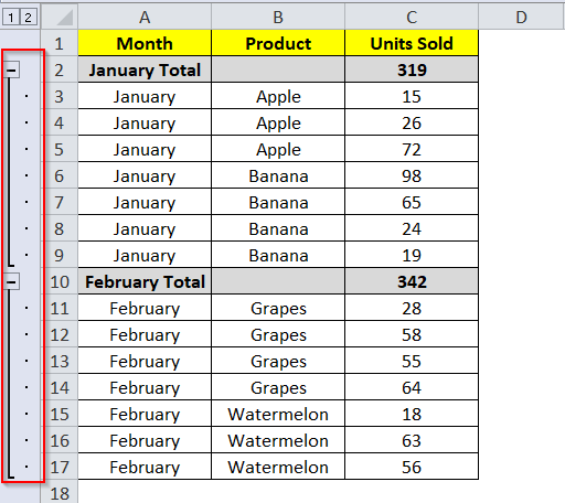
As now the subtotals are above the data, therefore, the direction of the groups has also changed accordingly.
Removing the Outline
Ungroup All At One Go
Click on the “Data” tab and go to the “Outline” group. Click on the arrow under the “Ungroup” option and select the option “Clear Outline”.

You would notice that all the groups get removed.
Ungroup only Certain Group of Rows
Follow the below steps to remove the grouping of only certain row groups without impacting the other groups:
Step 1: Select the rows that you want to Ungroup.
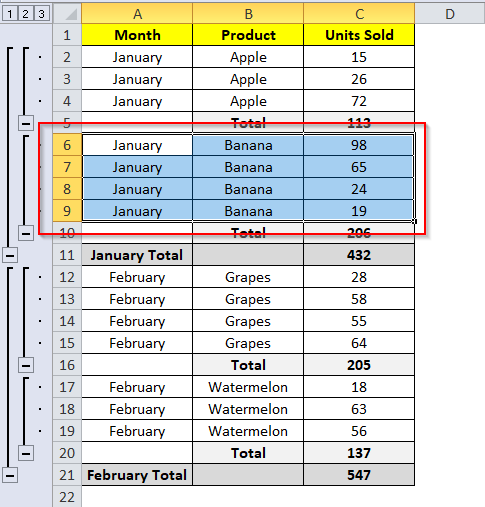
Step 2: Follow the path: “Data” tab > “Outline” group > ‘Ungroup’ button.

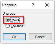
The “Ungroup” dialog would appear.
Step 3: Select the radio button “Rows” and click on the “OK” button.
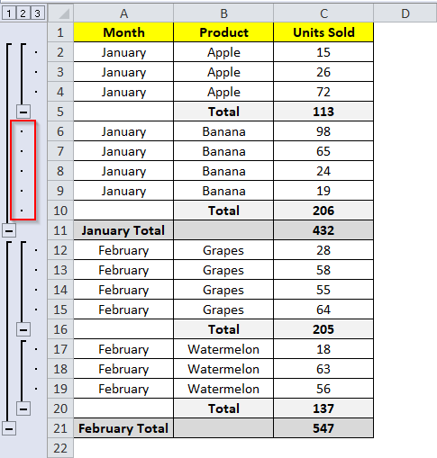
This would Ungroup the selected rows without impacting the other groups.
This brings us to the end of this blog. Share your views and comments in the comment section below to improve.
