Stack Data from One Column into Multiple Columns

You may have often faced a situation while working in an Excel Worksheet that you have all the in the single-column which should ideally be in the form of a table (into multiple columns). Converting this single column data into a table format by simply copying the cell and pasting it into a table format under the correct table heading is very time consuming and you would never like to do it. So what is the solution to quickly stack the data in one column into multiple columns. In this blog, we would unlock this technique to convert the data in one column into the readable table format.

Let us first understand what do we exactly mean by stacking the data from one column into multiple.

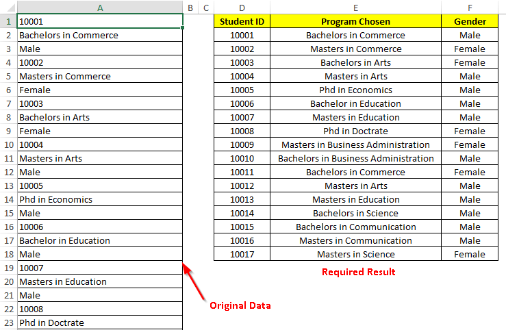
Suppose you have an excel worksheet in which the data (that ideally should have been in the form of a table) is in a single column. Now you want this data in a single column to get converted into a table.

There is an example in the screenshot below. In column A, we have the Student ID in the first cell, Program Chosen in the next cell followed by Gender in the third cell. The same repeats for the second student ID. You now want to organize and structure this data in a table format.

Let us now unlock this amazing trick which can make your task very easy.

Refer to the section below to stack the data available in a single column into a table format (to make it meaningful).

How to Stack Data from One Column to Multiple Columns

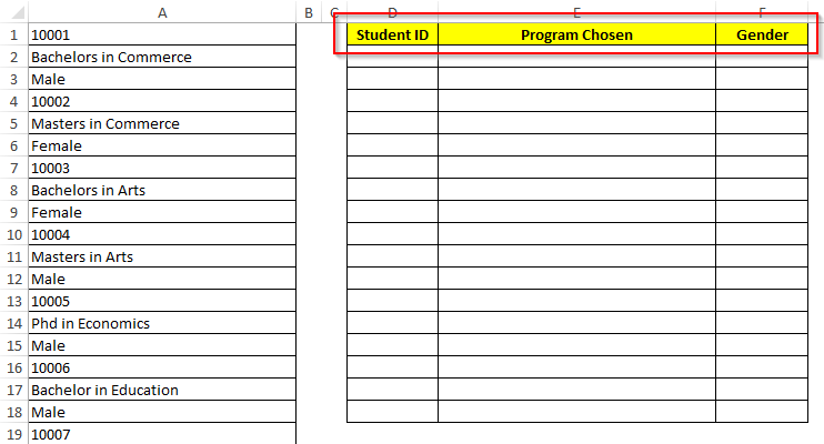
Firstly, enter the column headings of the required table as shown in the screenshot below:

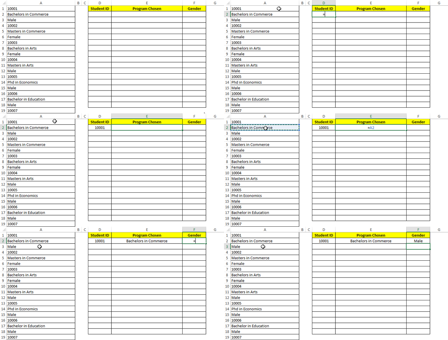
Now, In cell D2, give reference to cell A1 (=A1). Similarly, in cell E2, give reference to cell A2 (=A2) and in cell F2, give reference to cell A3 (=A3).

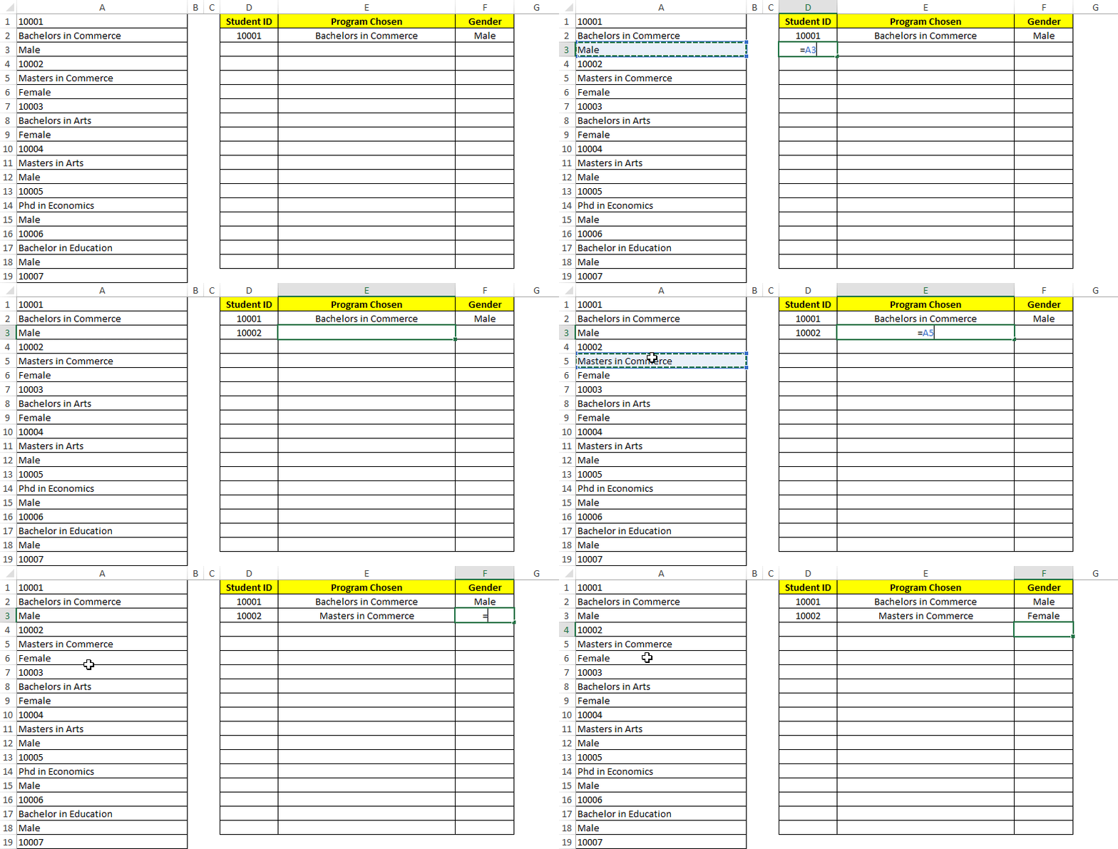
Again perform the above step for the second student ID. Give reference to the second student in the second row of the table as demonstrated below:

Now select the two rows of the table, and open the “Find and Replace” dialog box using “Ctrl+H” on your keyboard.

In the “Find What” section of this dialog box, enter ‘=’ sign and in the “Replace With” section, enter any character of your choice. I have entered the word ‘EU’ representing ‘Excel Unlocked’ :).

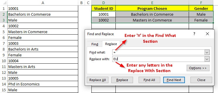
Now Click on the “Replace All” button. You would notice that your values in the table changes to ‘EU’ followed by the cell reference.

Hover your mouse to the bottom-right corner of the selected cells until mouse cursor changes to a plus symbol.

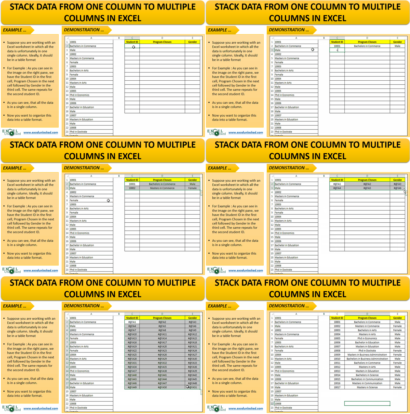
Now left-click on your mouse and drag the mouse downwards till the row you feel your data exists. I know that there are 17 students, therefore, I have dragged the mouse cursor till that limit. 

Release the mouse cursor once you have reached the last row.

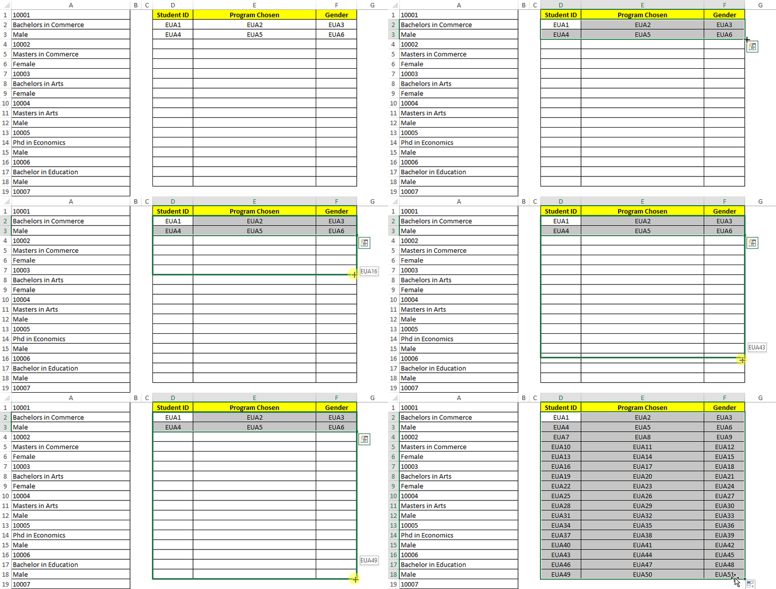
Again select the data table and press Ctrl+H on your keyboard to open the “Find and Replace” dialog box.

In the “Find What” section, enter ‘EU’ and in the “Replace With” section enter ‘=’. Now click on the “Replace All” button.

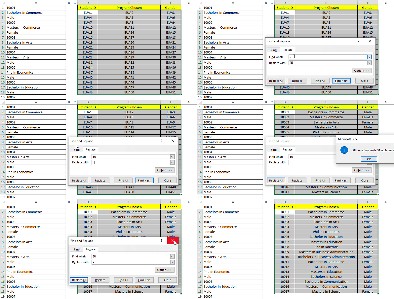
As soon as you press the “Replace All” button, you would notice that the data which was in one column is now available in a structured way in the form of a table.

This brings us to the end of this blog.