Generally, tables in Excel have headings on the top (i.e. column headings). In that case, it is very easy to sort the data from top to bottom. But, many a time, you may a table where the headings are on the left of the table. That means instead of the column heading, you have row headings. You cannot sort by the rows in excel directly. Then, how can you achieve this? In this tutorial, we would learn to sort the table by rows in Excel. To sort the table from left to right, we need to first make some changes in the settings so that excel can sort the table from left to right.
Sample Data Table (with table heading as row headings) :

Changing Orientation of Sorting
Follow the below steps to sort the data from left to right:
Step 1: Click any cell on the data table.
Step 2: Go to the “Data” tab. In the “Data & Filter” group, select the “Sort” button as shown in the screenshot below :

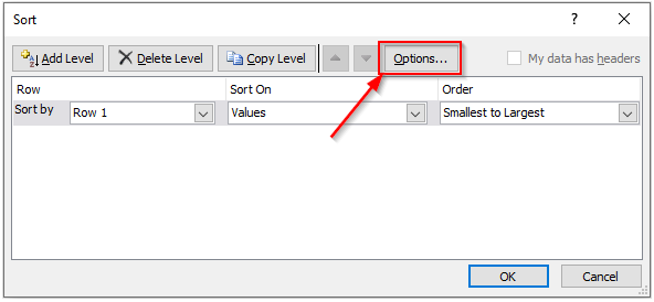
The “Sort” dialog box would open.
Step 3: In the “Sort” dialog box, click on the “Options” button.

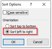
Step 4: You would notice that the “Sort Options” pop up box would appear on your screen.
Select the radio button “Sort left to right” and click on the “OK” button.

With this, you have changed the orientation of sorting. Now we are ready for sorting the data in Excel.
Sort Rows from Left to Right in Excel
To sort the table from left to right, refer to the steps below:
Step 1: Firstly, select the dataset. But do not select the headings (A1:A3).
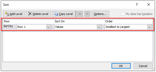
Step 2: Under the heading “Row”, select the row number by which you want to sort your data.
Suppose I want to sort my data by “Customer key”, i.e. row 1, therefore, select the option “Row 1” from the drop-down menu.
In the “Sort On” heading, select the option “Values” from the drop-down options.
And in the “Order” heading, select the option “Smallest to Largest” to sort the data in ascending order or “Largest to Smallest” to sort the list in descending order.
Also Read: How to Sort a Table or Data in Excel

As soon as you click on the “OK” button, you would notice that the entire table is now sorted based on the “Customer Key”.
This brings us to the end of this blog.

