How to Sort Pivot Table Manually?

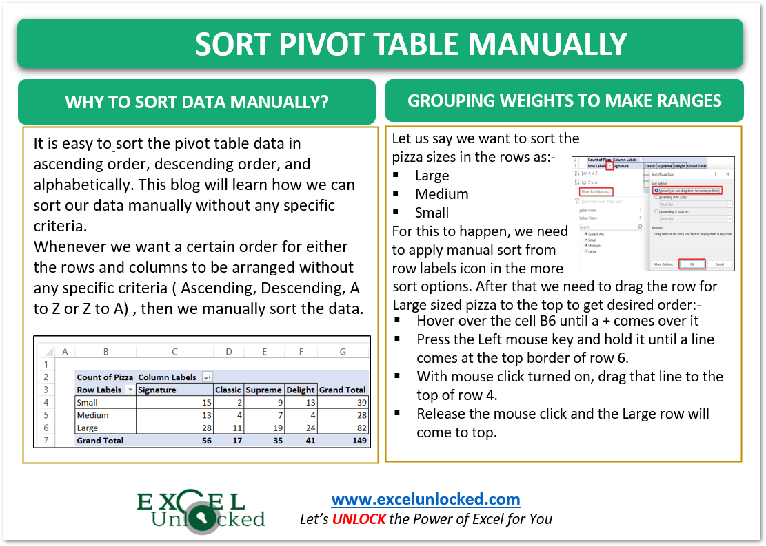
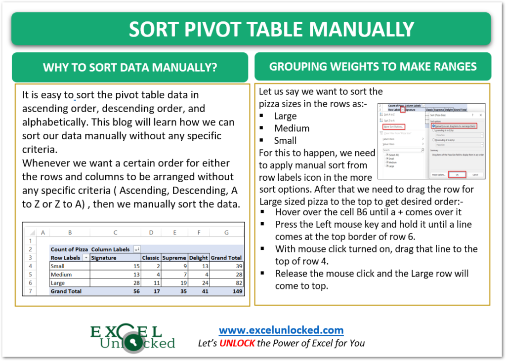
In the previous blog, we learned how to sort the pivot table data in ascending order, descending order, and alphabetically. This blog will learn how we can sort our data manually without any specific criteria. So let’s get started.

Example of Pivot Table for Sorting Data

Let us say we have the sales of pizzas divided into Pizza Category and Pizza Size. Following are the pizza categories available in the shop.

• Classic
• Delight
• Signature
• Supreme

And along with this, the pizzas were available in three different sizes as follows:-

• Small
• Medium
• Large

Moreover, we have made a pivot table representing the total number of pizzas sold for different category pizzas available in three pizza sizes.

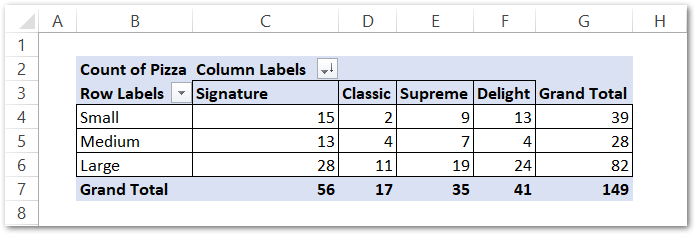
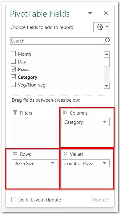
Here we have the Category in Columns Section, Size in Columns Section, and Pizza Count as Values.

Sorting the Rows Manually

Let us say, we want a specific order for the rows containing pizza sizes as follows:-

• Medium ( first )
• Large ( second )
• Small ( third )

Enabling the Manual Sort in Pivot Table

This is neither an A to Z sort nor a Z to A sort, which makes us manually sort the pivot table data in this case. However, to manually sort the rows:-

• Click on the button next to Row Labels in cell B3.
• Click on More Sort Options from there and choose the Manual Sort option.

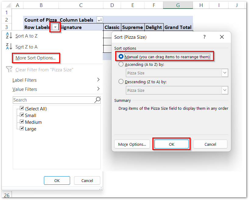
• This opens the Sort Dialog box for Pizza Sizes. Choose the first option for Manual Sort.
• This enables the Manual Sort and now we need to actually manually sort the pivot table rows.

Manually Sorting the Data

We would now drag the rows to make them follow the required order. The first step is to take the Medium-Sized pizza row from the 5th row of the sheet to the 4th row of our spreadsheet. Run the following steps to do this:-

• Hover the cursor on cell B5 ( containing the Medium ) until the cursor changes to a + sign like this.

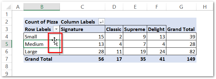
• Now make a Left mouse click and hold on to it.

• A straight line will appear above the row that you want to order. Now with the left mouse click being held, simply move your cursor to one row above. The line will come above the 4th row.

• Now release the mouse click. You will see that the entire data for Medium-Sized Pizza has come in the top row ( 4th row ) as follows.

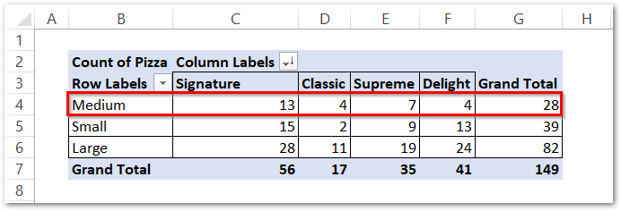
Also, the Small-Sized pizza row has shifted one row below.

Similarly, you can change the order for the Large-Sized Pizza row from the 6th row to the 5th row. Consequently, the Small-Sized Pizza row will again shift one row below as shown in the results.

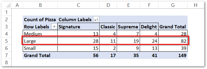
As a result, we have achieved the required sort order for our pivot table rows.

Manually Sorting the Fields ( columns ) of a Pivot Table

We have got the Pizza Categories in the columns. Let us say we want to change the Order of the categories ( from left to right ) to:-

• Classic
• Signature
• Delight
• Supreme

All you need to do is:-

• Drag the Column for Classic ( D3 ) to one column at its left. This will replace Column C with Classic and Columb D with Signature.
• Drag the Column for Supreme ( E3 ) to one column right to it. This replaces Column F with Supreme and Column E with Delight.

Consequently, this brings us to the end of the blog.

Thank you for reading 😊