Text and Number Filter in Pivot Table in Excel

There are a number of ways to filter the data in a pivot table. In the previous blog, we learned how to filter the pivot table data using Slicers. This blog will cover the Text and Number filter in Pivot Table that we can apply directly to the pivot table data.

Let us see how they work!

What are Text and Number Filters?

As the name must have suggested to you, the Text Filter applies to the Text while the Number Filter goes for filtering the numerical values.

Once we apply a new filter, the previous filter is automatically removed.

There are many different types of Text and Number Filters available in excel as shown in the figure below.

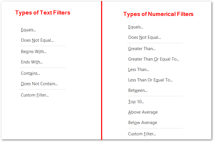
We have an option for Custom Filter available for both the Text Filters and Numerical Filters.

Taking a Pivot Table to apply Filters

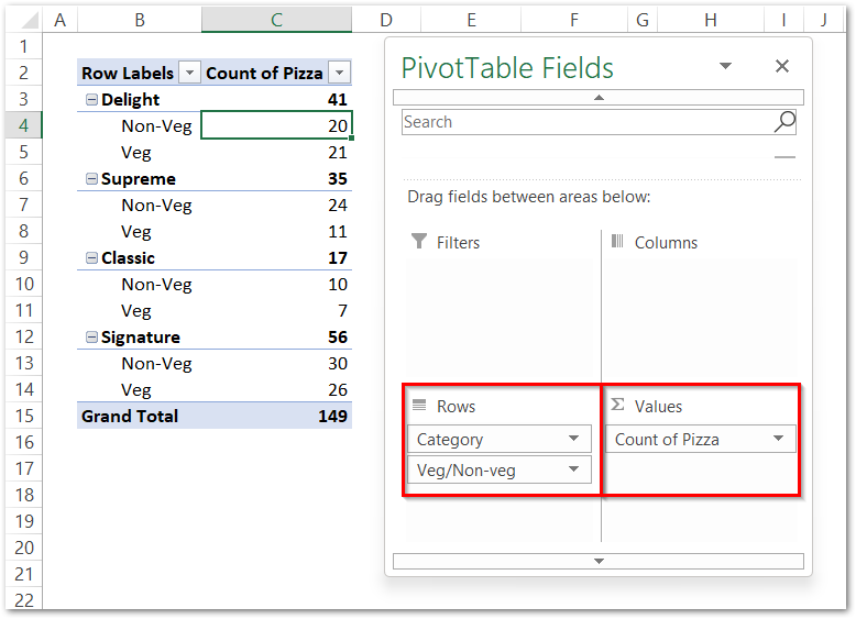
We have already learned about making a pivot table in excel. Let us say we have the count of pizzas sold, divided into Pizza Categories ( Delight, Supreme, Classic, and Signature ) and then further sub-divided the Pizza Categories into Veg and Non-Veg Pizzas.

Example 1 – Applying Number Filter on Pivot Table in Excel

Let us say we want to see those rows in our pivot table, for which pizzas were sold less than 20 in total. To do this:-

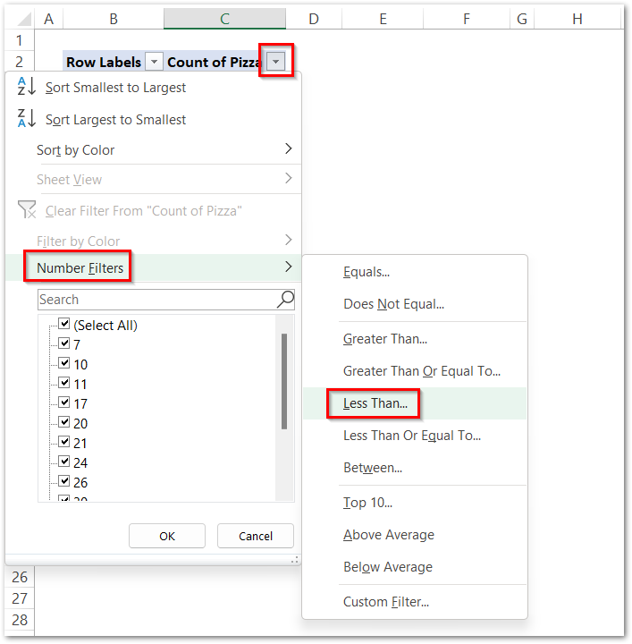
• Click on the button in cell C3 containing the Count of Pizza.
• Go to the option for Number Filters and then choose the Less Than.. Criterion.

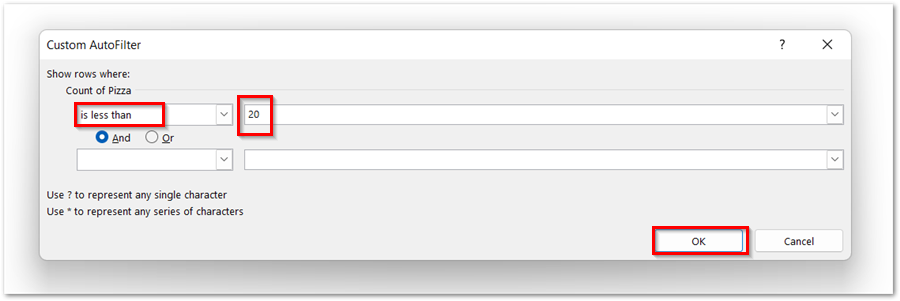
• This opens the Custom Filter Box. Set the value 20 in the Value less than field and then click ok.

As a result, the pivot table now displays the pizzas for which the corresponding value of the pizza count was greater than 20.

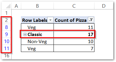
You can see that the Subtotal for the Categories ( Classic ) has been filtered out since the total sales for Classic Category Pizzas were less than 20.

Also, the groups have been removed and we cannot see directly that these veg and nonveg belong to which pizza category.

To know the pizza category, just hover the cursor over the cell.

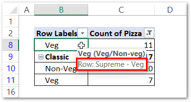
Also, you can see here that the row numbers are not sequential. This is so because those roses that didn’t meet the filter criteria ( not less than 20 pizza count ) were hidden.

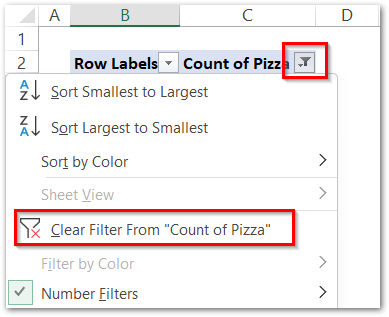
We can remove this filter from the Filter button in cell C2.

Example 2 – Applying Text Filter to Pivot Table

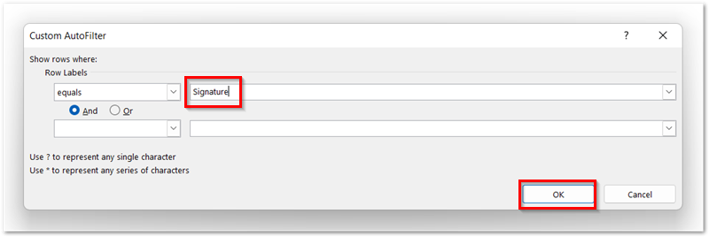
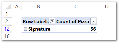
Let us say we want to see the sales of Signature Category Pizzas only, For this, we need to apply a Text Filter since “Signature” is a text string. To do this:-

• Click on the button in cell B2 next to Row Labels.
• Choose the Text Filters from the many and select Equals Filter Criterion.

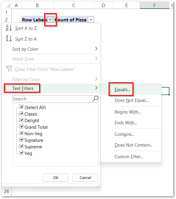
• Type Signature in the Text Equals Field and click ok.

This gives us the filtered results as follows.

In a similar way, we can apply other types of Text and Number Filter to the pivot table.

This brings us to the end of the blog.

Thank you for reading.