There are several ways to filter our data in the pivot table. Since pivot tables use the simplest drag and drop field method, slicers are also the easiest to use with a pivot table.
We can also connect single slicers to multiple pivot tables having the same pivot cache.
When to use Slicers with Pivot Table in Excel?
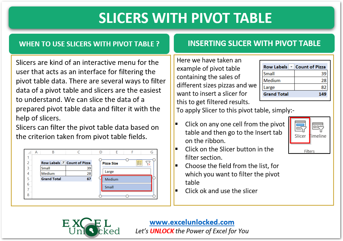
Slicers are kind of an interactive menu for the user that acts as an interface for filtering the pivot table data. There are several ways to filter data of a pivot table and slicers are the easiest to understand. We can slice the data of a prepared pivot table data and filter it with the help of slicers.
Slicers can filter the pivot table data based on the criterion taken from pivot table fields.
We can link one or more slicers to a single pivot table and then choose what selective (filtered ) information we want from our pivot table.
Example 1 – Single Slicer for Pivot Table
We have already learned to make a pivot table in Excel In this example, we are taking a pivot table representing the sales of different sized pizzas of a shop as follows.
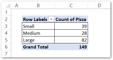
Here we want to apply a filter on this by getting the sale for only one ( or multiple ) pizza sizes sale at a time. To add a slicer to this pivot table:-
- Click on any cell in the pivot table and then go to the Insert Tab on the ribbon.
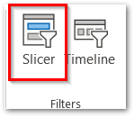
- Hit the Slicer button in the Filter Group.
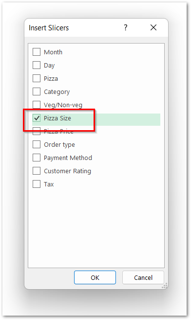
- A list containing all the fields ( columns ) from the pivot table’s source data will appear.
- Mark the pizza size from there and click ok.
- This inserts a slicer containing a button for all the pizza sizes in the pizza size column of our pivot table data. The slicer would be linked to our pivot table as we selected a cell from the pivot table before inserting the slicer.
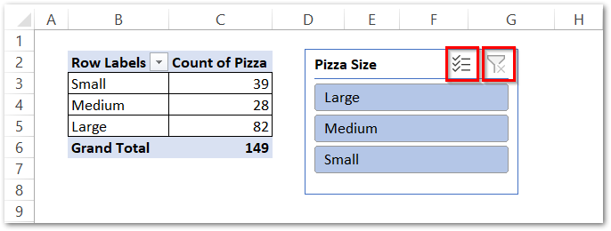
Buttons in the Slicer ( Multiselect and Remove Filter )
You can see that there are two buttons on the top of a slicer. Let us understand what they are for.
- Multi-Select – This is used to toggle the mode to select the multiple pizza sizes and not to filter the results only for one pizza size. For example Pizza count of Small and Large-sized pizzas.
- Clear Filter – This removes the selections we have made in our slicer and sets it to no selection, consequently removing the filter on the pivot table applied by that slicer
So right now if we Click on the Large button on our slicer, this is what happens.
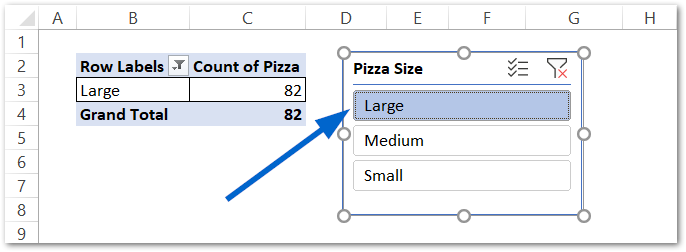
And if we press the Alt S key ( shortcut to turn on multi-select ), we will be able to choose different pizza sizes to filter. Unselect the Large and select Medium and Small Size pizza on the slicer.
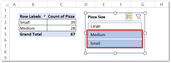
As a result, the pivot table shows the data for Medium and Small Size Pizza only. To get back to the unfiltered pivot table, simply press Atl C ( shortcut for clearing the filter ).
Example 2 – Multiple Slicers for Pivot Table
Each Slicer can contain the selection buttons from only one field ( column ) of our pivot data. For example, one slicer can give us the filtered results for the sales of January. We will need a separate slicer to filter the results for Sales in the First week.
When we want to apply a filter based on multiple criteria, then comes the use of Multiple Slicers. We can insert two slicers with different fields for one pivot table.
Let us suppose that we have the number of pizzas sold as follows:-
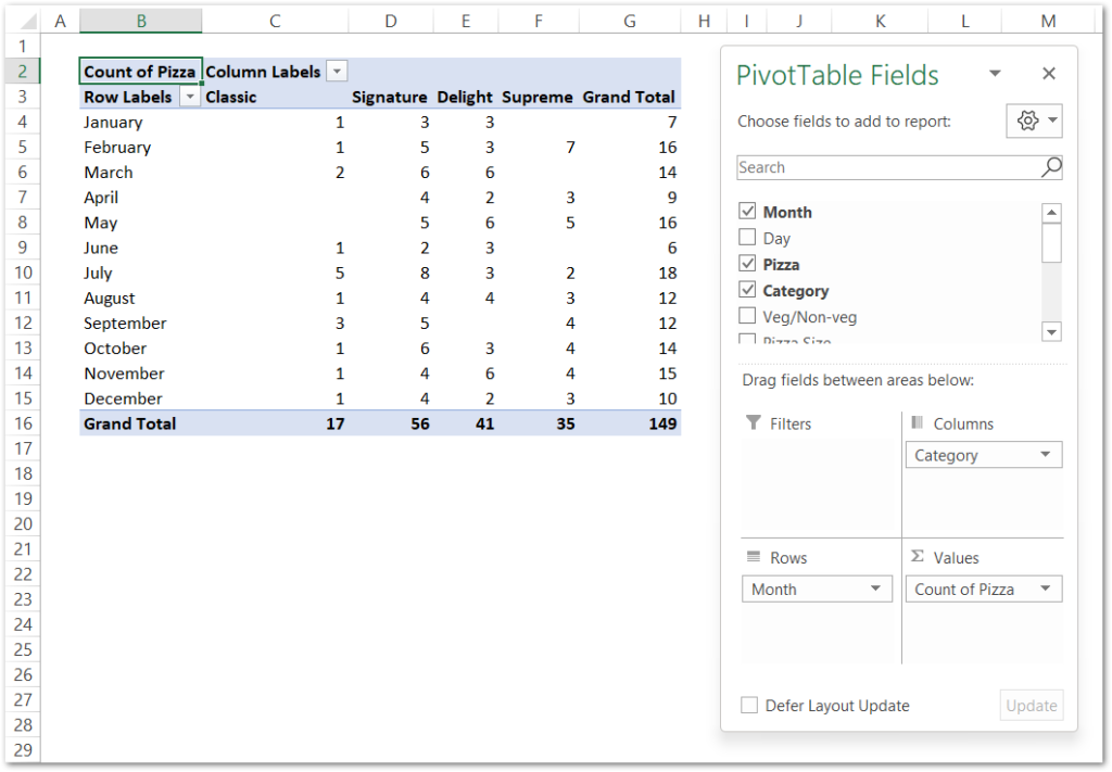
The data is divided into months (rows) and Categories ( Columns ).
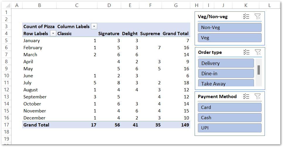
Insert a slicer as mentioned in example 1, but select the Order Type, Veg/Non-Veg, and Payment Method.
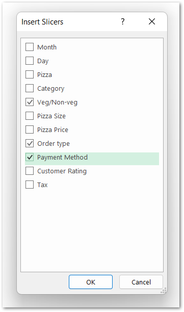
Click ok and then adjust the position of the slider.
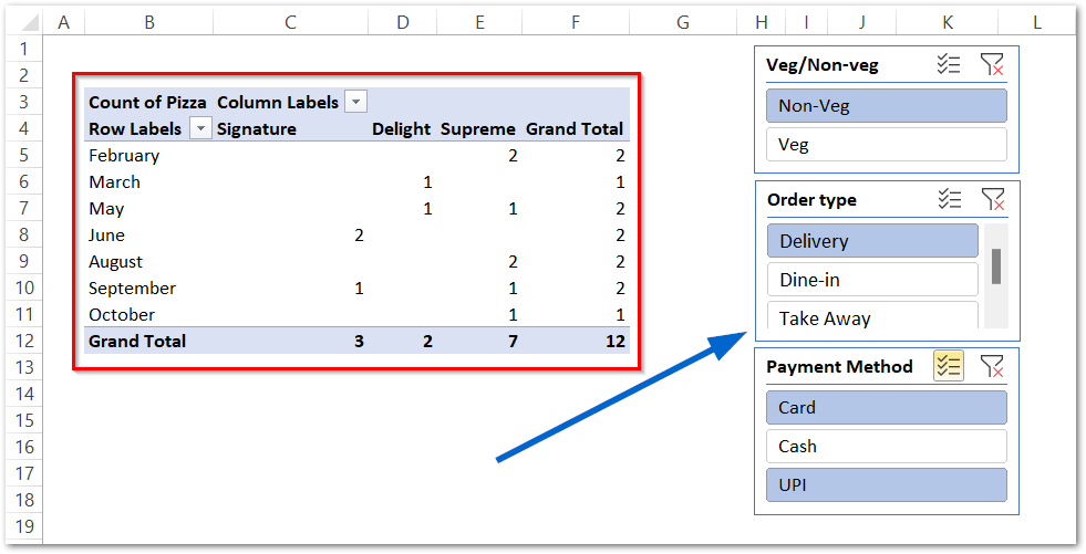
Now we can get the sales for Non-Veg ( Veg/Non-Veg) Pizzas that were delivered ( order type ) by Card and UPI ( payment methods ).
This brings us to the end of the blog.
Thank you for reading.

