We can use slicers with a pivot table to apply filters on the inserted pivot table. A pivot table timeline is also an important tool using which we can apply a type of filter to it.
Let us see how this works.
What is a Pivot Table Timeline?
The pivot table timeline lets us filter the pivot table based on the dates. We can filter the data lying in between a certain period of time. This period can be in days, months, quarters, or years based on your choice.
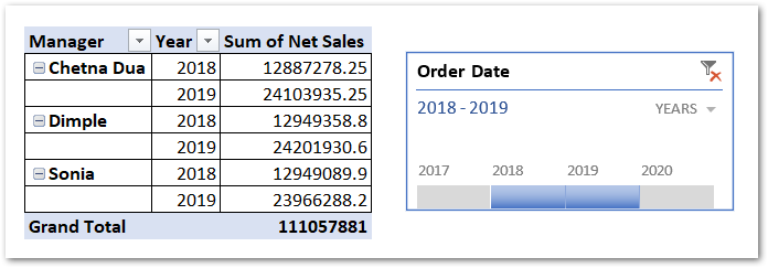
How to Add a Pivot Table Timeline in Excel?
A Pivot table timeline can be added to a pivot table that has at least one field in date format to apply the timeline on. Let us suppose we have the
Let us suppose we have a pivot table containing sales for different types of food items for years 2017,2018,2019, and 2020 years as follows:-
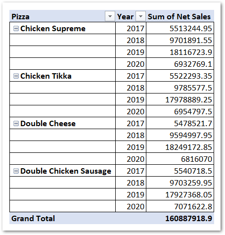
To add a timeline to this pivot based on the date on which the order for the food item was placed, we need to follow the below-mentioned steps.
- Click on any cell in the pivot table.
- Go to the Pivot Table Analyze tab on the ribbon.
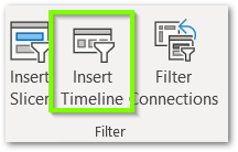
- In the Filter Group, click on the Insert Timeline Button.
- Choose the field name from the list of fields based on which you want to insert the timeline. Only the field having date format would be shown here.
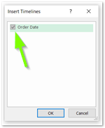
This is going to insert a default timeline in the worksheet containing the pivot table.
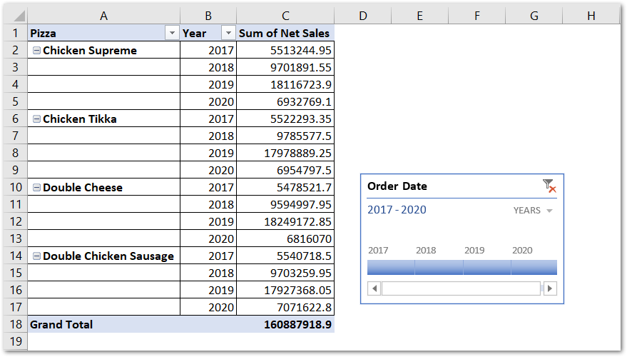

Working with Timeline
We have got a timeline inserted in the worksheet. Now we will learn about using a timeline.
Filtering Data for a Period of Years
We can find the sales of pizza from 2017 to 2018 and set the time period in the timeline.
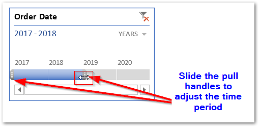
This would automatically filter the pivot table to show the sales of orders placed in the years 2017 and 2018.
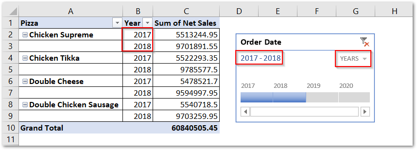
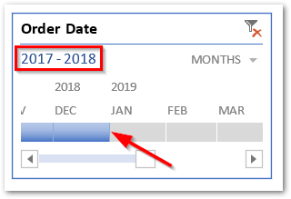
The top left corner displays the period for which data is filtered. Here it is 2017-2018. We can also filter the data based on months, quarters, or days.
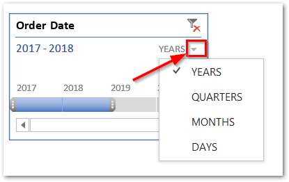
If we choose months, then we would be able to filter the data based on months.
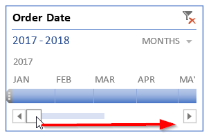
However, you can use the scrollbar at the bottom of the timeline to scroll to the months on the left or right. Since we filtered the data for the years 2017 and 2018 ( from the yearly timeline ), the monthly timeline would appear with the filter applied for 2017 and 2018.
Also Read: Slicers with Pivot Table – Multiple Slicers
Removing the Filter from Pivot Table
You can remove the filter applied by the timeline using the clear filter button at the top of the timeline.
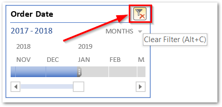
Moreover, you can use the shortcut to set the timeline to default is the Alt + C key. This is also going to remove the filter on the pivot table.
Formatting a Pivot Table Timeline
We can customize the appearance of a timeline in the following way.
- Select the timeline and go to the Timeline tab on the Pivot table.
- In the Styles group, you can alter the Pivot table appearance.

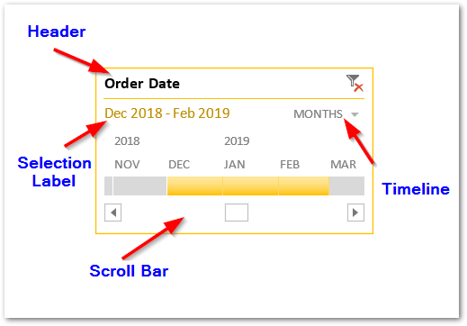
- Thereafter, you can also use the following options in Show Group to either show or hide the Timeline components.
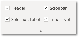
Unchecking the checkbox would hide the respective timeline component.
Deleting the Pivot Table Timeline
To delete the timeline:-
- Click on the Clear Filter Button on Timeline.
- Select the timeline and press the delete key.
This brings us to the end of the blog.
Thank you for reading.
