How to Change the Default Layout of a Pivot Table in Excel

A pivot table is used to get the summarized form of the data. In this blog, we would learn how to change the default layout of a pivot table.

Method of Changing Default Layout

Whenever we are inserting a pivot table, some settings are assigned to its layout by default. We can change the default settings of the pivot table using two methods.

• Import settings from an existing layout and make it as the default layout settings for the newly inserted pivot tables.
• Change the default settings to directly customize as per the requirement.

Whenever, we change the default layout settings in a pivot table, the layout changes are not observed in the existing pivot tables in the opened spreadsheet. However, the settings are updated for all the new pivot tables thet we insert after changing the settings.

Customizing the Default Layout in Pivot Table

The path that leads to settings for customizing the Default Layout of newly inserted pivot tables is as follows. File tab < Options Menu < Data Tab < Edit Defaul Layout Button.

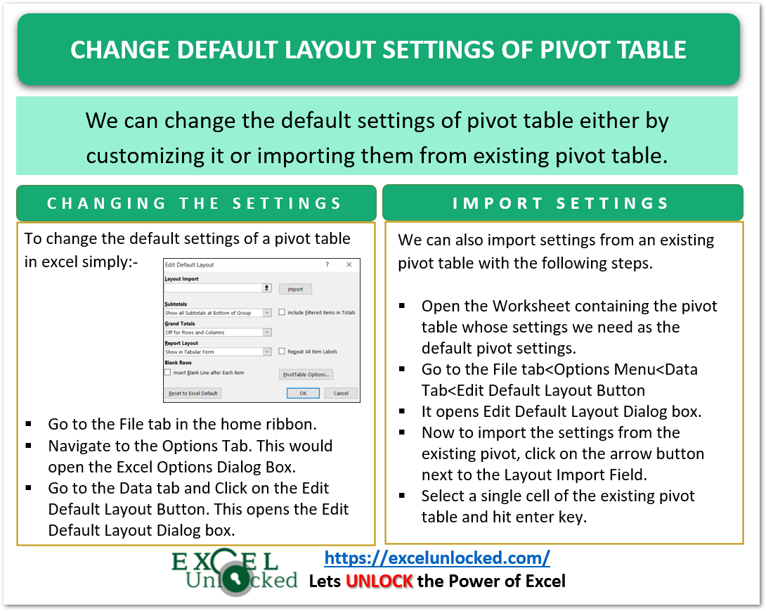
• Step 1 – Go to the File Tab on the ribbon at top.

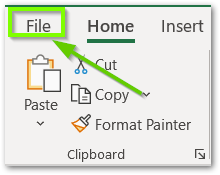
• Step 2 – Navigate to the Options Tab. This would open the Excel Options Dialog Box.

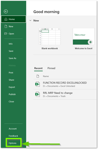
• Step 3 – Go to the Data tab and Click on the Edit Default Layout Button. This opens the Edit Default Layout Dialog box.

The Edit Layout Dialog Box is as follows.

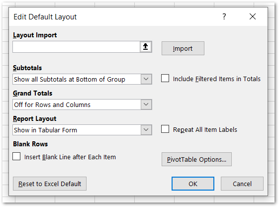
The following Points define the available settings for changing the default pivot table layout.

• Subtotals – This option allows us to change the default settings for the subtotals. We have three choices to choose from.

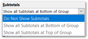
Once we change the settings and then insert a new pivot table, the subtotals settings would be applied to it.

• Grand Totals – This would change the visibility of grand totals for the rows and columns.

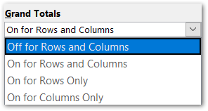
• Report Layout – This helps us to change the default layout of the pivot table. There are three available layouts.

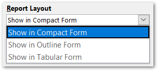
The following are the different layouts of pivot tables.

Importing the Settings from Existing Pivot Table

We can import the settings from the existing pivot table to be the default setting of all the pivot tables inserted thereafter.

All you need to do is:-

• Open the Worksheet containing the pivot table whose settings we need as the default pivot settings.
• Go to the File tab<Options Menu<Data Tab<Edit Default Layout Button

This opens the Edit Default Layout Dialog box.

• Now to import the settings from the existing pivot, click on the arrow button next to the Layout Import Field.
• Select a single cell of the existing pivot table and hit enter key.

This is all done.

With this, we have come to an end.

Thankyou for reading