This is the seventh tutorial of the Free ExcelUnlocked Pivot Table Course. In this tutorial, we would learn about multiple ways to manually refresh an excel pivot table.
Background
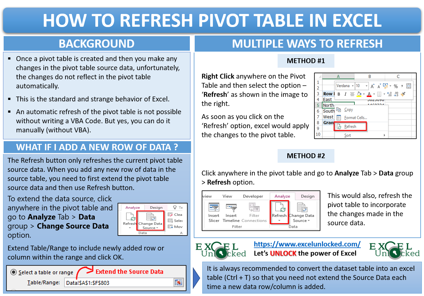
Once a pivot table is created and then you make any changes in the pivot table source data, unfortunately, the changes do not reflect in the pivot table automatically.
This is the standard and strange behavior of Excel. The pivot table does not automatically change or refresh itself when source data is changed.
So, what is the solution to this weird excel behavior? An automatic refresh of the pivot table is not possible without writing a VBA Code. But yes, you can do it manually (without VBA), see below:
Multiple Ways to Manually Refresh Pivot Table in Excel
As mentioned above, you need to refresh the pivot table manually to update the changes made in source table data to the pivot table.
There are three ways to achieve this as stated below:
- Right-click anywhere on the pivot table and select the option ‘Refresh‘, as shown in the image below:

- Another way is to use the ribbon options to refresh the pivot table. Click anywhere in the pivot table and go to Analyze Tab > Data group > Refresh option. See image below:

- The last way to instantly refresh the pivot table in excel is to use the keyboard shortcut – Alt + F5.
However, when you insert any new row of data to your dataset, before refreshing, you also need to change and extend the source of the data.
To extend the data source, click anywhere in the pivot table and go to Analyze Tab > Data group > Change Source Data option.

In the dialog box that appears, extend the Table/Range so as to include the newly added row or column within the range. Once extended, finally click on OK.

The coolest way to get rid of changing the pivot table data source, again and again, is by converting the dataset into an Excel Table. To do this, click anywhere on the dataset and press keyboard shortcut Ctrl + T. The ‘Create Table’ dialog box would appear wherein make sure to tick the checkbox ‘My Table has headers’ and then click OK. Now, if you add any row or column in this table, it would expand automatically and accommodate the new row/column. And now, there will be no need to extend the source of the pivot table.
Check out other Excel Pivot table related blogs on Free Pivot Table Course by Excelunlocked.