Apply Conditional Formatting to Excel Pivot Table

In this part of the Free ExcelUnlocked Pivot Table Course, we would learn about how to apply conditional formatting in the Pivot Table in Excel.

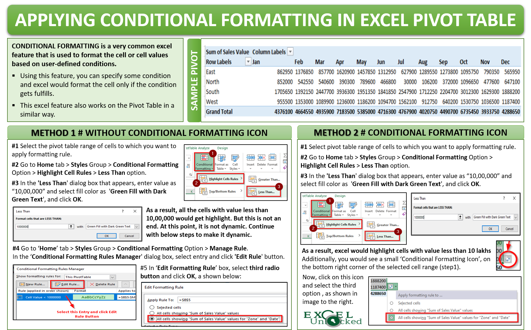
Conditional Formatting is a very common excel feature that is used to format the cell or cell values based on user-defined conditions. Using this feature, you can specify some condition and excel would format the cell only if the condition gets fulfills. This excel feature also works on the Pivot Table in a similar way.

Before we start, click on the Download button to get the sample excel file with a created pivot table.

Let us now begin with this tutorial and unlock multiple ways.

Applying Conditional Formatting in Pivot Table

In this sample pivot table, let us fill the cells color with dark green if the value is less than 10,00,000.

There are two ways to apply conditional formatting to an excel pivot table. Let us check on both of these ways one by one.

Method 1 : Without Using Conditional Formatting Icon

Check and perform the below steps to apply conditional formatting without using formatting icon:

• Select the range of cells to which you want to apply the conditional formatting (which in our case is B5:M8).

• Now, Go to the Home tab > Styles Group > Conditional Formatting Option > Highlight Cell Rules > Less Than. See image below-

• In the ‘Less Than‘ dialog box that appears, enter the value as 10,00,000 and select the fill color as ‘Green Fill with Dark Green Text’, and click OK.

Apparently it looks that the values less than 10,00,000 are highlighted with green color

But this is not an end. If you try to add any new record to the source data and refresh the pivot table, excel would not apply the conditional formatting to the newly added record.

To perform dynamic conditional formatting, proceed with the below steps.

• Keep the cells selected and navigate to the path – Home tab > Styles Group > Conditional Formatting Option > Manage Rule.

• In the ‘Conditional Formatting Rules Manager‘ dialog box, simply select the entry and click on the ‘Edit Rule‘ button.

• In the ‘Edit Formatting Rule‘ dialog box that appears, select the third radio button and then click OK, as shown below:

Now, your conditional formatting is a dynamic one. If you add any new records to source data, excel would automatically apply conditional formatting to the new records.

Method 2 : By Using Conditional Formatting Icon

This is a more easy method to apply automatic conditional formatting to pivot table when any new record is added in source data. Basic steps remain the same as below:

• Select the range of cells to which you want to apply the conditional formatting (which in our case is B5:M8).

• Now, Go to the Home tab > Styles Group > Conditional Formatting Option > Highlight Cell Rules > Less Than. See image below-

• In the ‘Less Than‘ dialog box that appears, enter the value as 10,00,000 and select the fill color as ‘Green Fill with Dark Green Text’.

• As soon as you click on the ‘OK’ button, excel would apply conditional formatting to the existing pivot table. Also, you would see a small icon on the bottom right corner, highlighted below. It is called – “Conditional Formatting Icon“.

• Click on this icon and you would see the three options. Without doing anything else, select the third option and that’s it.

One of the limitations of the conditional formatting is that if you edit or change any of the pivot table row/column fields, the existing conditional formatting would vanish away. You have to then again apply the conditional formatting.

Check out other Excel Pivot table related blogs on Free Pivot Table Course by Excelunlocked.