Have you ever faced with a need to make your excel dataset table banded? By branded table, I mean that every second, third, fourth, etc. row is colored. You may feel with this need when you want to group your data in the blocks of 4, or 5, or 10, and so on and so forth. In this blog, we would unlock the technique to highlight every alternate row in excel i.e. every second row in the Excel dataset. You can use the same technique to highlight the rows at any interval. To highlight every alternate row, we would use the conditional formatting functionality of excel.
Let us begin with this technique.
Sample Dataset Table
Suppose we have a sample dataset as shown in the screenshot and the purpose here is to highlight alternate rows (i.e. Rows 3, 5, 7, 9 and so on)
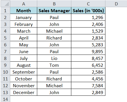
Highlight Alternate Rows in Excel
Consider the below step by step procedure to achieve the objective:
Step 1: Firstly, select the dataset (A2:C13) as demonstrated in the screenshot below :
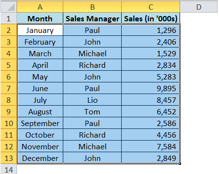
Step 2: Go to the “Home” tab and click on the option “Conditional Formatting”. You can find this option under the ‘Styles’ group

Step 3: From the drop-down options under the “Conditional Formatting”, select the option “New Rule”
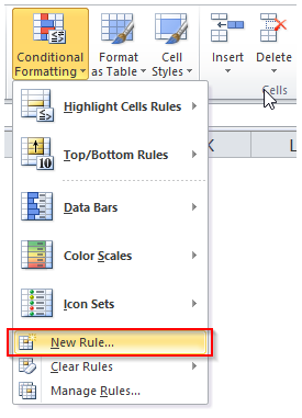
As a result, the “New Formatting Rule” dialog box will open.
Step 4: In the “Select a Rule Type” section of this dialog box, select the option “Use a formula to determine which cell to format” from the list of rules. As soon as you select this option, you would notice that an input box appears in the lower half of the dialog box.
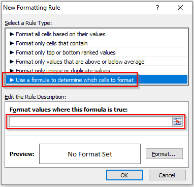
Step 5: In the input box as highlighted in the screenshot above, write the below formula :
=MOD(ROW($A2)-1,2)=0
Then, click on the “Format” button to open the dialog box – “Format Cell”.
In the “Format Cell” dialog box, go to the tab “Fill” and select the color of your choice from the range of colors. Additional colors are also available. You can find those by clicking on the button “More Colors”.
I have chosen Yellow color.
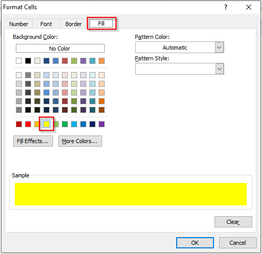
Finally, click “OK”.
This would take you back to the “New Conditional Formatting” dialog box. There as well, click the “OK” button to exit and activate the set conditional formatting.
Result
You will notice that the alternate rows in the dataset got highlighted with yellow color.
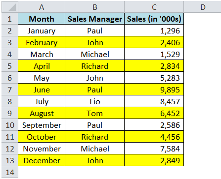
Similarly, if you want to highlight every third row, then, in that case, all the steps as explained above remain the same. Just the formula will change =MOD(ROW($A2)-1,3)=0.
As a result, every third row in the dataset gets highlighted.
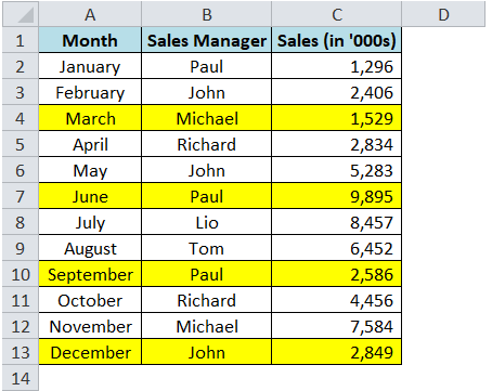
This brings us to the end of this blog. I hope that you have found this blog useful. Please share your valuable views and comments in the comment section below.

