In the previous blog, we learned the basics of conditional formatting. Today we would learn how to apply multiple conditional formatting rules on the same range of cells.
So let us begin learning.
Applying Multiple Conditional Formatting Rules
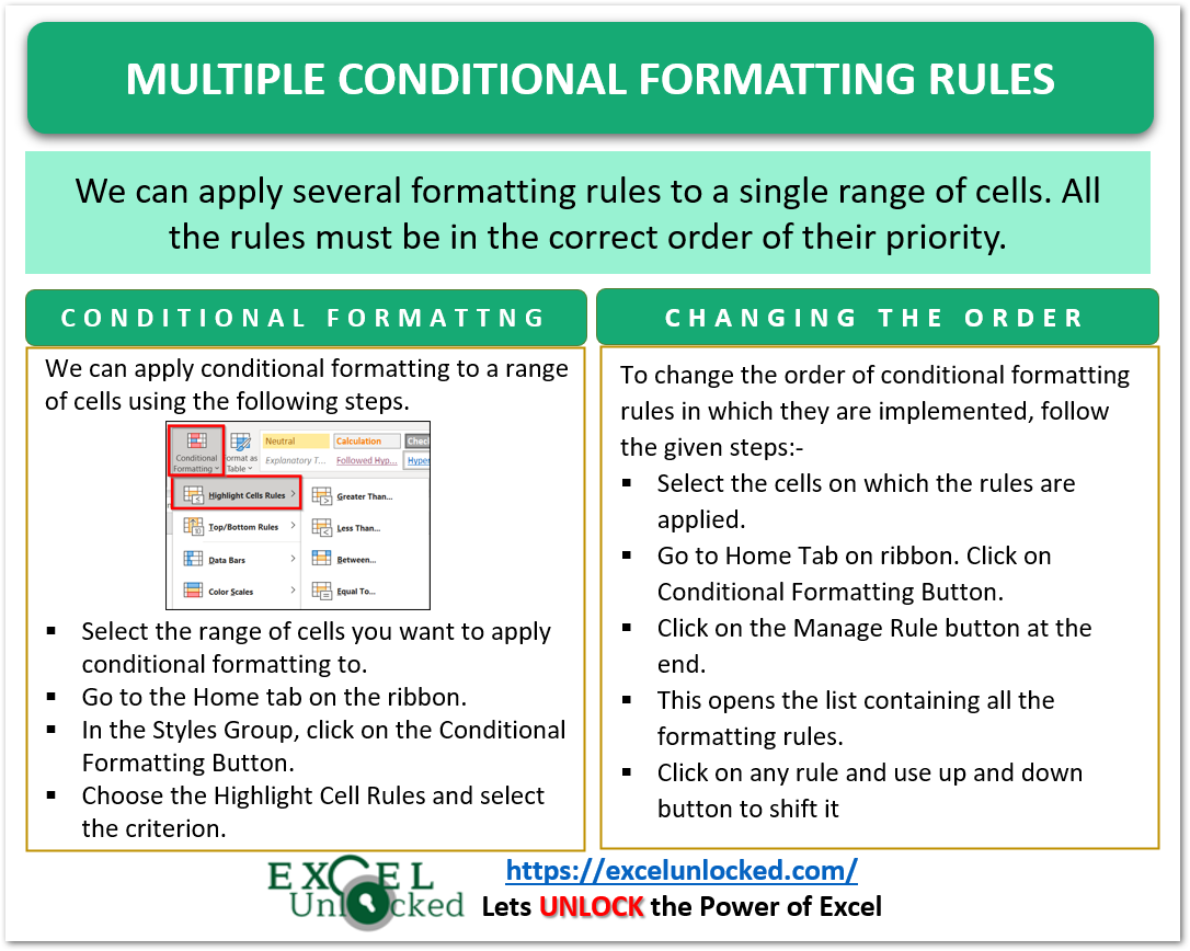
We can apply several formatting rules to a single range of cells. All the rules must be in the correct order of their priority.
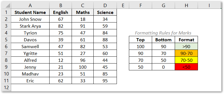
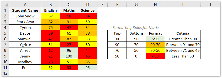
Let us suppose we have the marks of different students in a class test out of 100 as follows. We want to apply multiple conditions on the marks as follows:-
- Marks > 90 are highlighted in green
- Marks between 70 and 90 are in orange
- Marks between 50 and 70 are in yellow
- Marks less than 50 are in red
So basically, we got four rules to apply to the marks range.
You can download the practice workbook from here to practice along with us.
Step 1 – Applying Multiple Formatting Rules
We can apply the four rules with the Greater Than, Between, and Less than criteria. First of all, we would start by highlighting marks > 90 with green color.
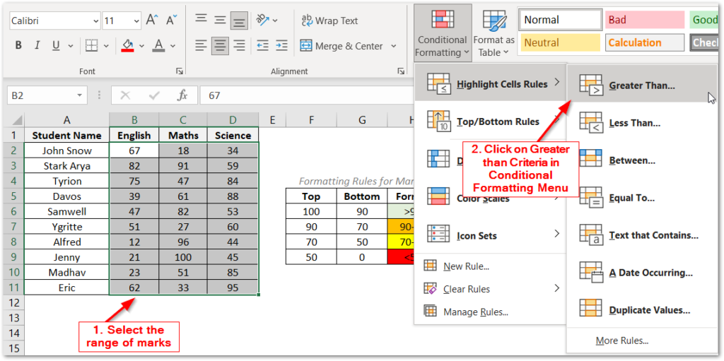
- Select the range of marks.
- Go to Home Tab>Conditional Formatting>Highlight Cells Rules>Greater Than
- Set the value for Criteria to be marks > 90. We would take the highlighted format as custom.
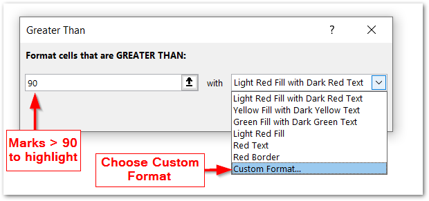
- Set the Custom Format to Green Fill Color.
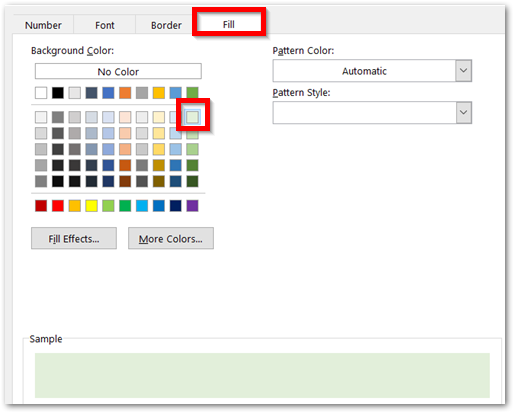
This formats the cells greater than 90 in green color.
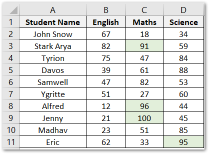
Similarly, we are going to apply three more criteria on this range of marks from the conditional formatting menu.
Step 2 – Priority of Criteria
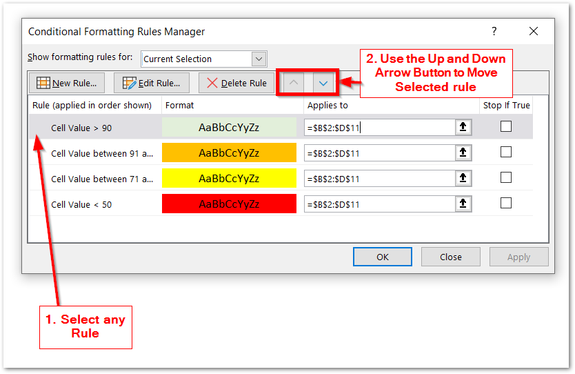
We need to set the different formatting rules in an order of priority. The rules are implemented in a fixed order. To change the order of rules:-
- Select any of the cells in the marks. Go to Home Tab> Conditional Formatting.
- Click on the Manage Rules button at the end.
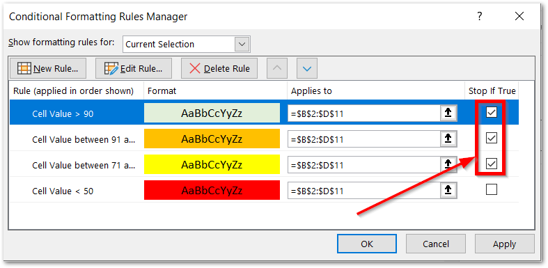
- Now change the order of rules to be the same as shown below. Use the arrow buttons to move a rule up and down on the priority list.
Step 3 – Stop if True
Stop if True is a conditional formatting rule property which means that if the conditional formatting rule is true for a cell, then the remaining formatting rules (that are below it in the order of implementation of the formatting rules list) will be disabled for that cell and would not be checked.
We would check all of them except the last rule.
This is all done.
Thank you for reading.
