Do you know, how to highlight the row that contains blank cells? In this blog, we would unlock the technique to highlight the complete row if any of the cells in that row contains any blank cells. Let me take one example to explain why you need to learn this trick. Let us suppose, you have asked your junior to enter the record of marks secured by students in various subjects in an Excel worksheet. Now, when your junior completes this task and provides you with the file, you find that there are many cells that are blank which is incorrect and you want to get the list of students for whom the marks have not been entered in the respective cell(s). So, in this case, you can highlight the complete row that contains even a single blank cell and then filter out the students based on the highlighted color.
To achieve this we would use the ‘Conditional Formatting’ functionality of Excel.
Sample Example Containing Blank Cells
The below is the screenshot which contains for country per year. As you can see from the dataset, there are few cells that are blank. The cells D3, G4, and B6 are blank and contain no data in it.

The task as you know here is to quickly highlight the rows that contain such missing figures.
Highlight Row Containing Blank Cells
As mentioned earlier, we would use the conditional formatting functionality of excel to highlight the complete row containing the blank cells.
Follow the below procedure to achieve the same.
Select the entire data set like the way it is shown in the screenshot below

In the ribbon bar, click on the tab “Home” and click on the option “Conditional Formatting” under the group ‘Style’.

From the drop-down options, click on the option “New Rules”.
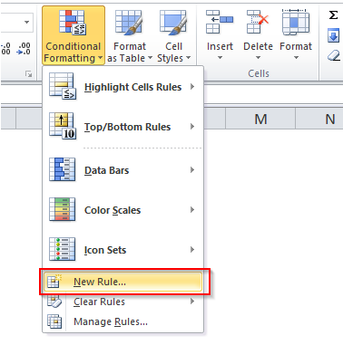
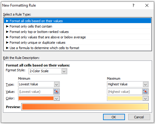
The “New Formatting Rule” dialog box would appear on your screen as shown in the screenshot below :
Under the “Select a Rule Type” section, click on the last option which says “Use a formula to determine which cells to format”.
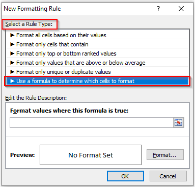
Here we would enter a formula to instruct excel to format the cell if the condition specified in the formula is TRUE.
Enter the following formula in the input box:
=COUNTIF($B2:$G2,””)>0
Instead, you can also enter =COUNTBLANK($B2:$G2)>0
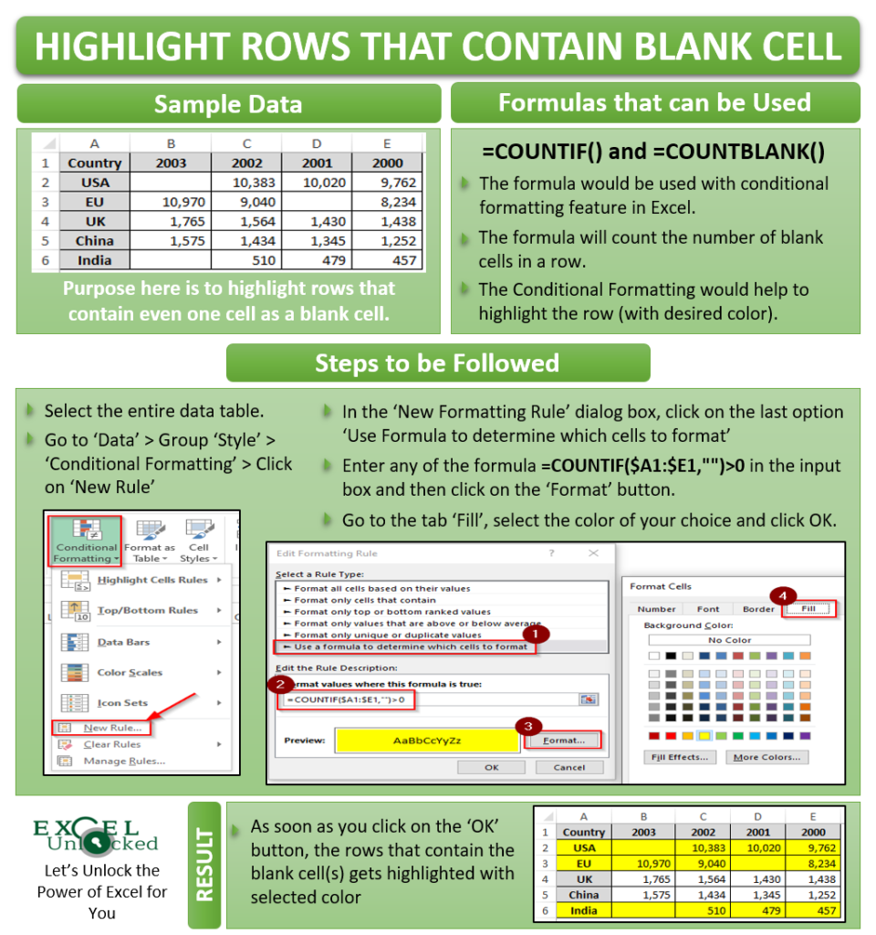
Now click on the “Format” button to open the ‘Format Cell’ dialog box. Under the “Fill” tab, choose the color of your choice from the available color, or you can also use other colors by clicking on the option “More Colors”.
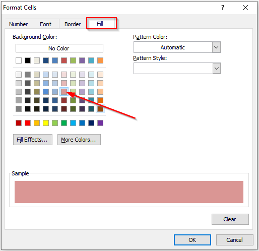
Finally, click OK to exit.
This brings us back to the “Conditional Formatting” dialog box. Here as well, click OK button.
As a result, you would notice that the rows that have even a single cell as a blank cell, would get filled with the selected color.
Also Read: What is Excel Conditional Formatting?

Now try to enter any number in cell G4 (at present it is blank).
What did you notice? The highlighted color disappears. This is because now, there is/are no blank cell(s) in row number 4.

Explanation of the Formula
The =COUNTIF($B2:$G2,””)>0 or =COUNTBLANK($B:$G2)>0 formulas count the blank cells in the rows. If the row contains any blank cell (i.e if the count of the blank cells in a row is more than 0), then the row gets highlighted with the selected color.
This brings us to the end of this blog. Share your views and comments in the comment section below.

