How to Sum Values Based on Criteria

In this blog, we would unlock the technique to sum the values in the range based on the criteria. It means that the excel would return the sum of the values (in the cell range) only if the criteria specified are fulfilled. There are two basic formulas to sum the values based on criteria which are: =SUMIF() and the other one is =SUMIFS().

The first formula =SUMIF() is used to sum the range of values if you want to check only for one criterion. The second formula =SUMIFS() is used where you want that Excel should check multiple criteria and perform the sum function if all the specified conditions or criteria are fulfilled.

In this blog, you would learn the =SUMIF() formula.

Purpose of =SUMIF() formula

This formula is used to conditionally sum values based on a single criterion. 

=SUMIF(range,criteria,[sum_range])

The first attribute of this formula is range. In this attribute, you need to select the range of cells that are evaluated for criteria.

The second attribute is the criteria where we need to specify the condition to be met.

Both the above attributes are mandatory attributes.

The third and the last attribute of this formula is sum_range. Here you need to specify the range of cells to be summed up if the criteria (the second attribute) is met or satisfied. This is an optional attribute and if it is omitted then excel would sum the same range of cells that are evaluated for condition fulfillment.

Sum Values Based on Criteria: Some Practical Example

As you can see from the above formula, the =SUMIF() formula only works if you want to check for a single condition. 

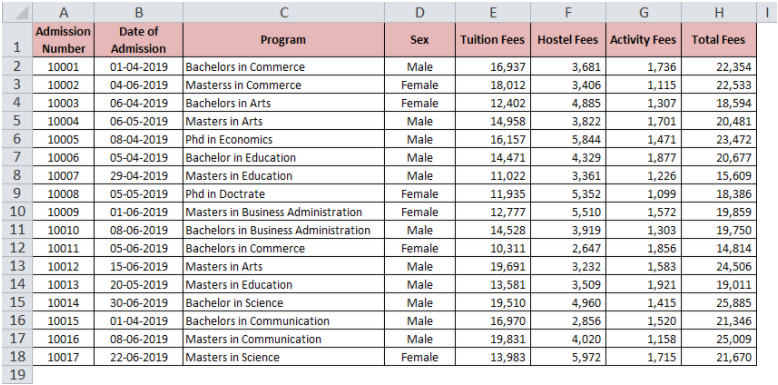
Look at the sample data table below. It contains some basic details about admission in the University like admission number, date of admission, program, Candidate Sex, tuition fees, hostel accommodation fees, activity fees, and total fees amount.

Now let us look at some amazing things that you can do using the Excel =SUMIF() function.

Example 1: Using =SUMIF() with Mathematical Operators

Let us now understand how to sum the values that are greater than or less than or equal to some value.

To find the sum of tuition fees if the tuition fees amount is greater than $15,000 enter the following formula:

=SUMIF(E2:E18,”>15000″,E2:E18)

As a result, you would get the sum value as 1,27,108.

Instead of entering the value in the criteria attribute, you can even give the cell reference. In that case, the formula would look like this:

=SUMIF(E2:E18,”>”&K2,E2:E18)

Similarly, you can use the less than operator (<) to sum only if the value is less than the specified value.

Enter the following formula to find the sum of activity fees if the amount is less than $1,500.

=SUMIF(G2:G18,”<1500″,G2:G18

Likewise, the equal to (=) operator can be used to find the sum of the value is equal to the specified value.

Other useful operators:

Less than equal to operator (<=): This operator returns the sum of values if the value is less than or equal to the specified value.

Greater than equal to operator (>=): This operator returns the sum of values if the value is greater than or equal to the specified value.

Not equal to (<>): This operator returns the sum of values only if the value is not equal to the specified value.

Example 2: Sum if using the Text Criteria

In addition to the number criteria as explained above, the =SUMIF() will also sum the range of values based on whether the criteria range contains the text or not.

Suppose you want to find the total fees amount for the male candidates.

Enter the following formula:

=SUMIF(D2:D18,”Male”,H2:H18)

As a result, you would get the sum of the total fees for the male students.

Instead of typing the criteria as “Male”, you can even give the reference of the cell as demonstrated below:

=SUMIF(D2:D18,K2,H2:H18)

To sum if the text is not equal to “Male”, use the not equal to operator (<>) as below:

=SUMIF(D2:D18,”<>”&K2,H2:H18)

This would give the sum of total fees amount if the gender is not “Male”.

Example 3: Sum if the corresponding cell has Partial Text Match

The wildcard characters are used to sum the values if there is a partial match in the text criteria or condition.

For example, suppose you want to sum the hostel fees amount if the program chosen is a graduation program. This means that the program chosen column must contain the word “Bachelor”.

To do such a partial match, we can use the asterisk character (*) in the criteria attribute.

Enter the following formula to sum the hostel accommodation fees amount if the program is a bachelor degree:

=SUMIF(C2:C18,”*”&”Bachelors”&”*”,F2:F18)

To use the cell reference along with wildcard characters, use the below formula

=SUMIF(C2:C18,”*”&K2&”*”,F2:F18)

Using ampersand (&) on either side of the cell reference concatenates the wildcard character and cell reference.

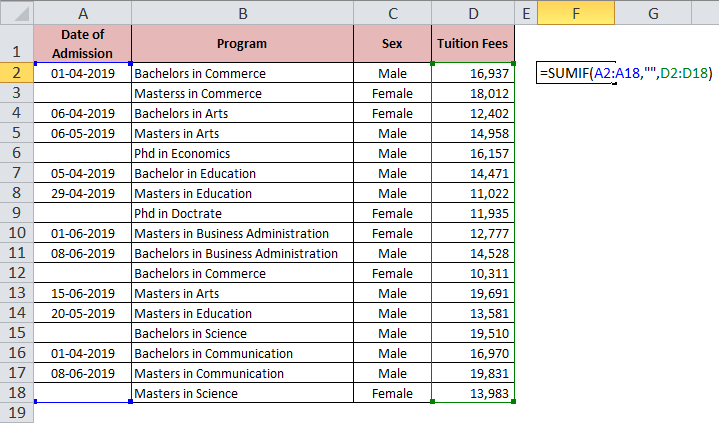
Example 4: Sum Cells that correspond to Blank Cell

To sum the values, if the corresponding cell is blank, enter the following formula:

=SUMIF(A2:A18,””,D2:D18)

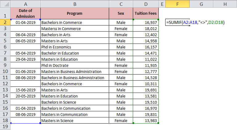
Example 5: Sum values based on cells that correspond to Non-Blank Cell

To sum the values, if the corresponding cell is not a blank cell, enter the following formula

=SUMIF(A2:A18,”<>”,D2:D18)

Example 6: Using =SUMIF() with dates

You can also find the sum based on the date as the criteria.

To find the sum based on a certain date, use formula:

=SUMIF(B2:B18,”01-04-2019″,H2:H18)

Similarly, you can use the =SUMIF() formula with other operators (>,<,<>,>=,<=, etc.)

This brings us to the end of this blog.