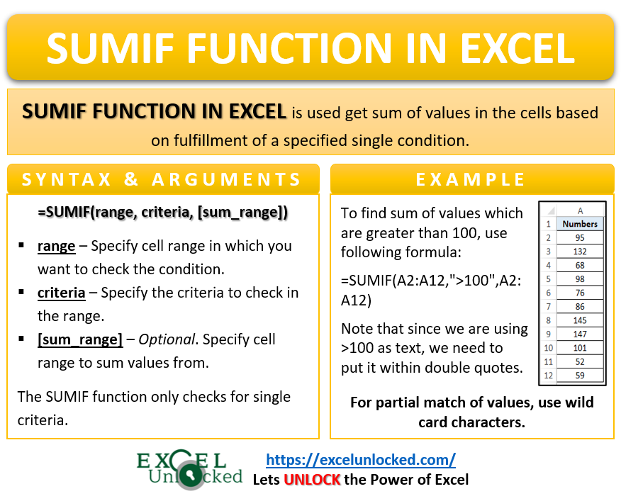
The Excel SUMIF function is a mathematical formula that is an advanced version of SUM function in excel.
The name in itself clarifies its purpose. SUM + IF meaning to find SUM of numbers in cell(s) only IF the specified condition is met.
In this tutorial we would learn about how to use the SUMIF function in excel, along with its syntax arguments and examples.
Here we go 😎
When to Use SUMIF Function in Excel
The SUMIF formula is a part of the math/trig function group. This formula used to get the total of numbers in the cells based on the fulfillment of a specified condition.
It is important to note that the SUMIF formula only checks for a single condition and not more.
It returns the sum of values.
Syntax and Arguments
=SUMIF(range, criteria, [sum_range])
Below points explain the arguments of the SUMIF function:
- range – In this argument, specify the cell range in which you want to check the condition.
- criteria – In this argument, specify the criteria to check in the range. This argument supports condition check by using logical operators like >,<,>=,<=, and =. It also supports the use of wildcard characters i.e. an asterisk (*) and question mark (?) for partial matches of values.
- [sum_range]) – This is an optional argument. In this argument, specify the cell range to sum values from. If you keep it blank, then the formula takes the [sum_range] (third argument) same as the criteria range (first argument).
To reiterate, the SUMIF function only checks for a single criteria. If you want to check for multiple criterias, then use the SUMIFS excel function.
Examples of SUMIF Function in Excel
Let us now learn with the help of examples about how the SUMIF function works in excel.
Ex. 1 # Sum Values Only If They Are Greater Than Or Less Than A Number
Suppose you have a list of numbers in excel and you want to find the sum of those numbers or values which are greater than 100.
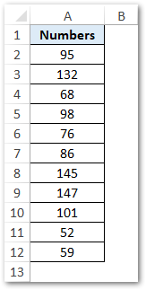
To do so, use the below formula:
=SUMIF(A2:A12,">100",A2:A12)
As a result, excel would total only those values from the range which are greater than 100.
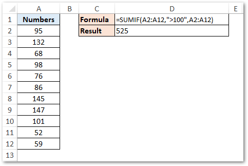
Note that, any text that you mention in the criteria argument must be specified without double quotes (” “). In above example, we have entered the text >100 within double quotes.
Instead of manually typing the criteria text, you may even use reference of a cell. In that case, do not use double quotes. See below image.
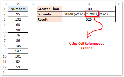
In the above example, to join the mathematical operator symbol and the reference cell, I have used the ampersand symbol (&). We may instead use the CONCATENATE excel function, like this:
=SUMIF(A2:A12,CONCATENATE(">",D1),A2:A12)Other mathematical logical operators are:
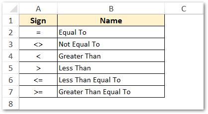
Ex. 2 # SUM Values Based on Text
In the above example we saw how to sum values based on the number criteria. In this example section, we would learn how to sum values based on the text criteria.
Also Read: How to Sum Values Based on Criteria
The below image shows the region wise sales made by a company in a year.
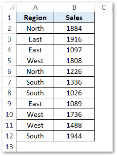
Suppose you want to find the total sales made in the West region. To achieve this, use the following formula:
=SUMIF(A2:A12,"West",B2:B12)
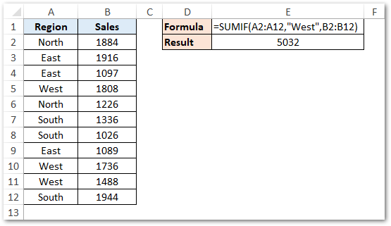
As a result, excel returns the value 5032 (which is total sales made in West.
Ex. 3 # SUM Values Using Partial Match of Text
Wildcard characters play a very important role in excel when you want to find and/or replace values based on a partial match of text. There are mainly three wildcard characters namely – asterisk (*), question mark (?), and tidle (~).
The below image illustrates the sales made by different companies spread across world. Here, IN – India, CA – Canada, FI – Finland, US – Unites States of America, and SE – Sweden.
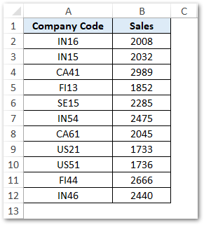
Now, to find the total sales made by all Indian company codes (starting with IN), the asterisk wildcard characters will be useful.
Use the following formula:
=SUMIF(A2:A12,"IN*",B2:B12)
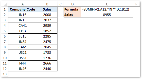
In the above example, the criteria “IN*” (an asterisk after IN) searches for all the texts in range A2:A12 which starts with the word IN.
To learn using wildcard excel characters in more detail, go to this link.
Ex. 4 # Working With Dates in SUMIF Excel Function
Using the SUMIF function, we can also find the sum of values that occur before or after a particular date. Or does not occur on a particular date.
Let’s see an example to understand the same. In the below example, we have a list of week days along with total hours worked by an employee during those days.
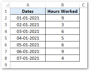
Suppose we want to find sum of total hours worked except on 06-01-2021.
To achieve this, use the following formula:
=SUMIF(A2:A8,"<>"&DATE(2021,1,6),B2:B8)
OR
=SUMIF(A2:A8,"<>"&B7,B2:B8)
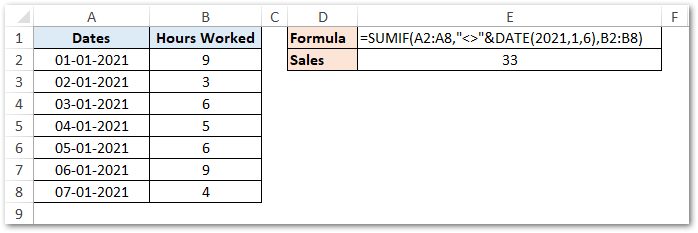
In the above example, since we want to exclude a single date, we have used the mathematical operator not equal to (<>).
Also, we have nested the DATE excel function inside the SUMIF function to return a date value.
This brings us to the end of this article on SUMIF formula in excel.
Thank You 🙂
RELATED POSTS
- SUM Function in Excel – Add All Numbers in Cells
- COUNTIF Function In Excel – Counting Cells With Condition
- Excel COUNTIFS Function – Counting Cells with Specified Conditions
- SUMPRODUCT Function in Excel – Usage with Examples
- AND Function in Excel – Check Multiple Conditions
- IF Function in Excel – Check Logical Condition
