Excel COUNTIFS Function – Counting Cells with Specified Conditions

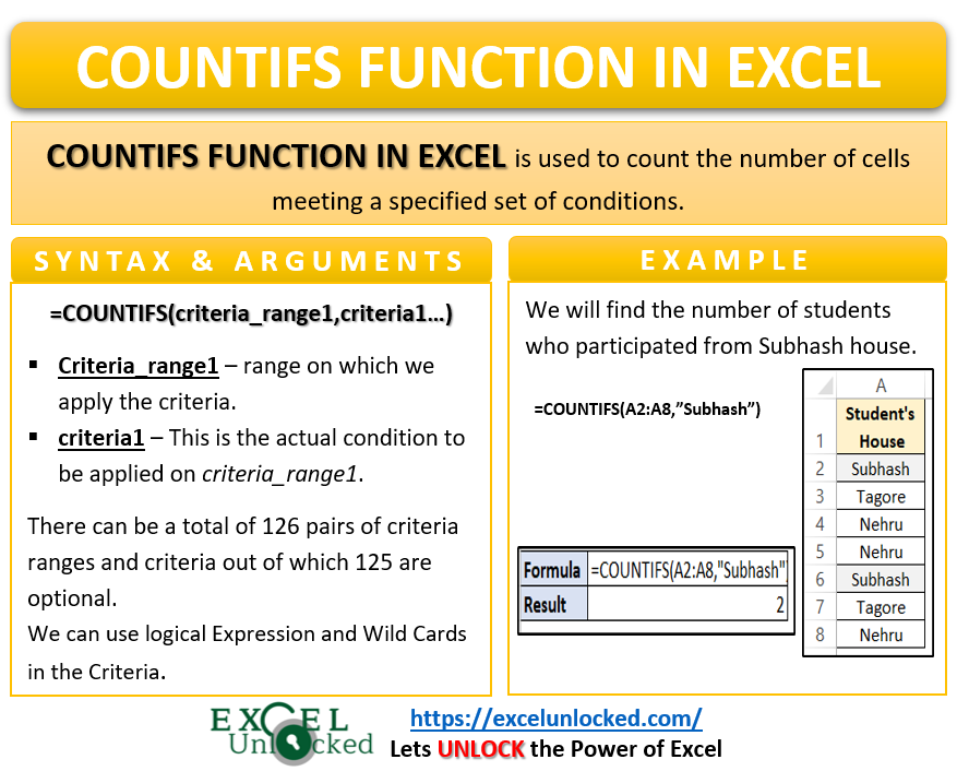
In one of our recent blogs, we used the COUNTIF function in excel to count the number of cells using one criterion. In this tutorial, we would learn how to use the COUNTIFS function in excel to count the number of cells if more than criteria (multiple criteria) gets fulfilled.

Here we go 😎

When to Use Excel COUNTIFS Formula

The COUNTIFS represents “Count cell ifs”. Here, “ifs” means there can be more than one condition. It is one of the basic statistical functions of Excel.

As mentioned earlier, the COUNTIFS function in excel is used to count the number of cells where more than one criteria fulfill simultaneously.

Syntax and Arguments

=COUNTIFS(criteria_range1,criteria1,[criteria_range2],[criteria2])

The below points explain the function arguments:

• criteria_range1 – In this argument, specify the range of cells to check for the first condition.

• criteria1 – In this argument, specify the condition to check on the criteria_range1.

• [criteria_range2] – This is an optional arguement. We will specify the second range if needed.

• [criteria2] – Specify the second condition to apply on criteria_range2.

There can be a maximum of 126 criteria ranges and their corresponding criteria. It is mandatory to specify atleast 1st criteria. The rest of the criterias are optional.

Must To Know Points About Excel COUNTIFS Function

The following points are important to know about the COUNTIFS function.

• It is not case sensitive.

• If you specify only one criteria, the function will work similar to the COUNTIF formula. (See example 1)

• The function uses AND logic if you specify multiple criterion. (See example 2)

• The function would return a zero if no cell satisfy the condition.

• We can use logical operators in the function criteria. While using the logical operators in COUNTIFS formula, make sure that,
  • The expression of a logical operator with a constant number must be enclosed within double quotes. For instance, “<80”.
  • The expression of logical operator with cell reference or other formula, the operator (<, >, <> ,=) will be enclosed in double quotes whereas the cell reference is concatened with the operator using an ampersand (&). For instance, “>”&A1 or “<”&TODAY().

• Similarly, you can even use the wildcard characters for fussy match of criteria. Use wild card characters when you have a rough idea over what you are finding in the range. Following wildcard characters are most used:
  • ? – for one missing character.
  • * – for a sequence of missing characters.

Examples to Learn COUNTIFS Function Of Excel

In this section, we would learn some of the examples for Excel COUNTIFS function.

Ex. 1 – Simplest Example For COUNTIFS formula of Excel

In this example of COUNTIFS function, let us start by taking the compulsory arguments.

The below image shows the information about scores in Inter-House Debate.

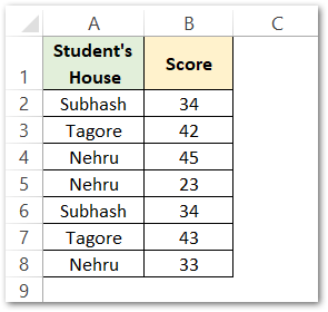
Let us say, we want to know the number of students who participated from the Nehru House. To achieve this, use this COUNTIFS Formula:

=COUNTIFS(A2:A8,"Nehru")

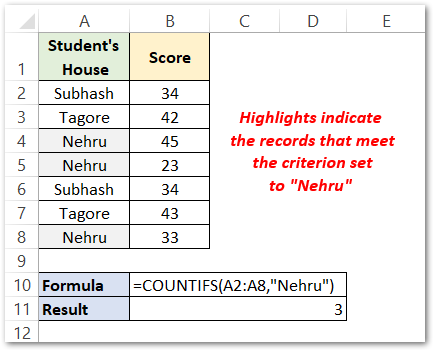
As a result, the function has returned 3.

Explanation – In the above example, the criteria_range1 is A2:A8 and the criteria1 is “Nehru”. This means that the function will search for the criteria “Nehru” in the range A2:A8. There are total 3 cells (A4, A5, A8) that contain the text string “Nehru”. Therefore, the result of the function is 3.

Ex. 2 – Using Multiple Criteria in COUNTIFS Function

Let us say there is a clothing company that supplies the cloth in meters. Below are its order details.

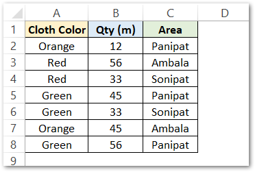
The owner wants to know how many customers bought green-colored cloths in Panipat.

You can see that there are two criteria to satisfy here. First – ‘Green’ color AND second – ‘Panipat’.

To achieve this, enter the following formula:

=COUNTIFS(A2:A8,"Green",C2:C8,"Panipat")

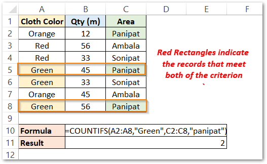
As a result, the function has returns 2.

Explanation – The first criteria “Green” applies to the range A2:A8. The corresponding cells satisfying this condition are in orange color. Similarly, the second criteria “Panipat” applies to the range C2:C8. The corresponding cells satisfying this condition are in Green color. After that, the function would use AND logic to check for the records that satisfy both of the criteria simultaneously (red-colored rectangle). The number of records that satisfy both of the conditions is 2. Hence, the formula returns 2 as its output.

Ex. 3 – Using Logical operator and Wild Cards in Excel COUNTIFS Function

Let’s suppose, the owner of a pet shop wants to know the number of customers who ordered more than one dog AND also had a pet dog.

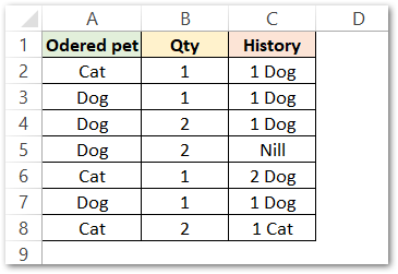
Use the following COUNTIFS Formula in Excel to get the required result.

 =COUNTIFS(A2:A8,"Dog",B2:B8,">1",C2:C8,"*Dog")

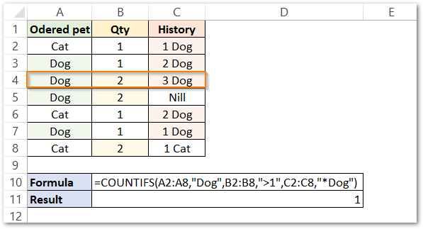
As a result, the function returns 1.

Explanation – In the above example, there are three conditions to be satisfied. The first condition “Dog” applies on range A2:A8. The cells containing the text string “Dog” are highlighted green. Likewise, the second condition “>1” applies on the range B2:B8. Orange highlights are the cells satisfying this criterion (i.e. value more than one). The third condition has a wildcard character “*Dog” (red highlights). Now the function follows the AND logic and counts the records that satisfy all of the three conditions simultaneously. There is only one such record (marked with a red rectangle. Therefore, the formula returns 1 as its output.

Thank you for Reading. 🙂