In the previous blog, we focused on understanding the basic usage of the SUMPRODUCT formula, its syntax and arguments, and some of the functions it replaces. Today, we will focus on some of the advanced applications of the SUMPRODUCT Function in Excel. We are assuming that you have a basic knowledge of this function or you can first understand the elementary usage.
Let’s jump to work.
Application 1 – Applying Multiple Criteria using SUMPRODUCT Function
Let us suppose we have the sales of the different vegetable orders as follows:-
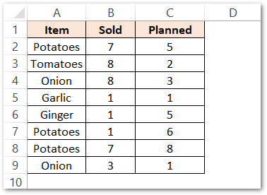
In this list, we want to count the number of orders placed for Potatoes for which the Sold were less than Planned. To do so, use the following SUMPRODUCT formula:-
=SUMPRODUCT(--(B2:B9<C2:C9),--(A2:A9="Potatoes"))
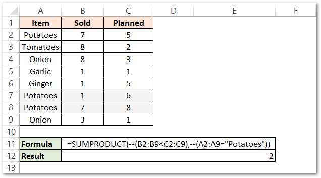
As a result, you can see that the formula has returned 2 as the total number of orders for potatoes for which the sold quantity was less than planned. The highlighted are the rows representing this information.
Explanation – We have passed two boolean arrays to the SUMPRODUCT formula and then used a double negative operator with them ( it converts the TRUE into 1 and FALSE into 0)
The boolean array supplied were:-
- B2:B9<C2:C9. In this, each cell of range B2:B9 ( Sold ) will be compared with C2:C9 ( planned ). A 1 will be returned if the condition is TRUE (sold<planned) and 0 if the condition is not satisfied ( sold>planned ). This returns a boolean array containing 8 values, one for each order:-
- A2:A9=”Potatoes”. This will compare each of the items in the range A2:A9 if it is equal to the string “Potatoes”. There will be a 1 or 0 returned for each of the 8 orders forming a boolean array.
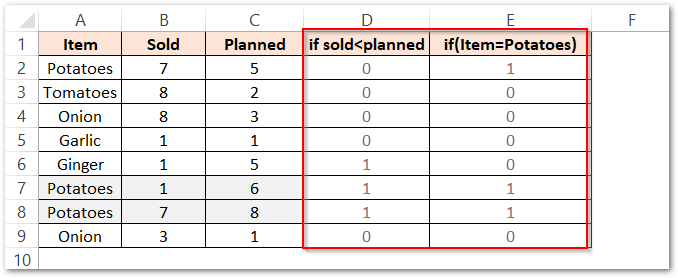
Now the SUMPRODUCT function will get the product of both the boolean arrays’ corresponding elements and then returns the sum as the count:-
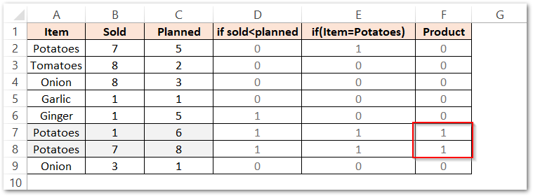
You can see that in the product column, we have the product of the boolean arrays in ranges D2:D9 and E2:E9.
=(D2*E2)+(D3*E3)+(D4*E4)+(D5*E5)+(D6*E6)+(D7*E7)+(D8*E8)+(D9*E9)
We got two 1 in cells F7 and F8 which means both the conditions are TRUE only for two rows.
So the function returned the count of orders for potatoes whose sold<planned as two orders.
So this was one of the applications of the SUMPRODUCT Function in Excel.
Application 2 – SUMPRODUCT to replace the SUMIFS Function
Let us say we have the above same list but with the order price column added with it as follows:-
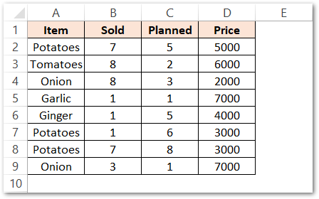
We want to get the Total Price for the order of Potatoes. This is when we can say we want the sum but with some condition applied. Use the following formula to get the sum of prices for the sales of potatoes.
=SUMPRODUCT(--(A2:A9="Potatoes"),D2:D9)
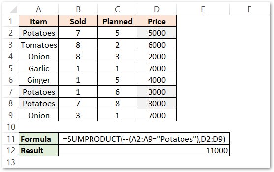
As a result, you can see that the function has returned 11000 as the total price for the Potatoes. Highlighted are the three rows containing sales for Potatoes ( 5000+3000+3000=11000).
Explanation – We have passed a boolean array ( set of TRUE (1) and FALSE (0) ) and a range of values as D2:D9 ( Price column ). The function will first check the condition for the range A2:A9 if it is equal to potatoes and return a boolean array of 1 and 0.
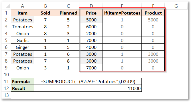
The range F2:F9 contains the boolean array. The second array is D2:D9. The function multiplies the two ranges F2:F9 ad D2:D9, the products are contained in the Product (F) column. The values in the range F2:F9 are then added to give the results as:-
=5000+0+0+0+0+3000+3000+0=11000
Application 3 – Lookup using the SUMPRODUCT Function
We can make a Lookup formula by using Excel’s SUMPRODUCT and EXACT Function. Let’s have a look at the merged syntax for both the functions to make it work like a lookup formula:-
=SUMPRODUCT(--(EXACT(Lookup_value,Lookup_range)),Return_Qty_Range)
The Return_Qty_Range can be numbers or magnitudes but not text strings as the SUMPRODUCT considers the text strings as zero.
Let’s have a look at the following example
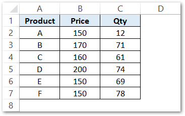
We want to find the Qty of Product D sold. So in this case the lookup value is “D” in the lookup range A2:A7. While we want to get the Qty for Product D ( Refer to cell E3), the Return_Qty_range is C2:C7.
=SUMPRODUCT(--(EXACT(E3,A2:A7)),C2:C7)
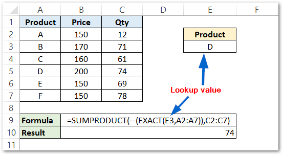
As a result, you can see that the formula has returned 74 as the Product D quantity.
This brings us to the end of the blog.
Thank you for reading.
