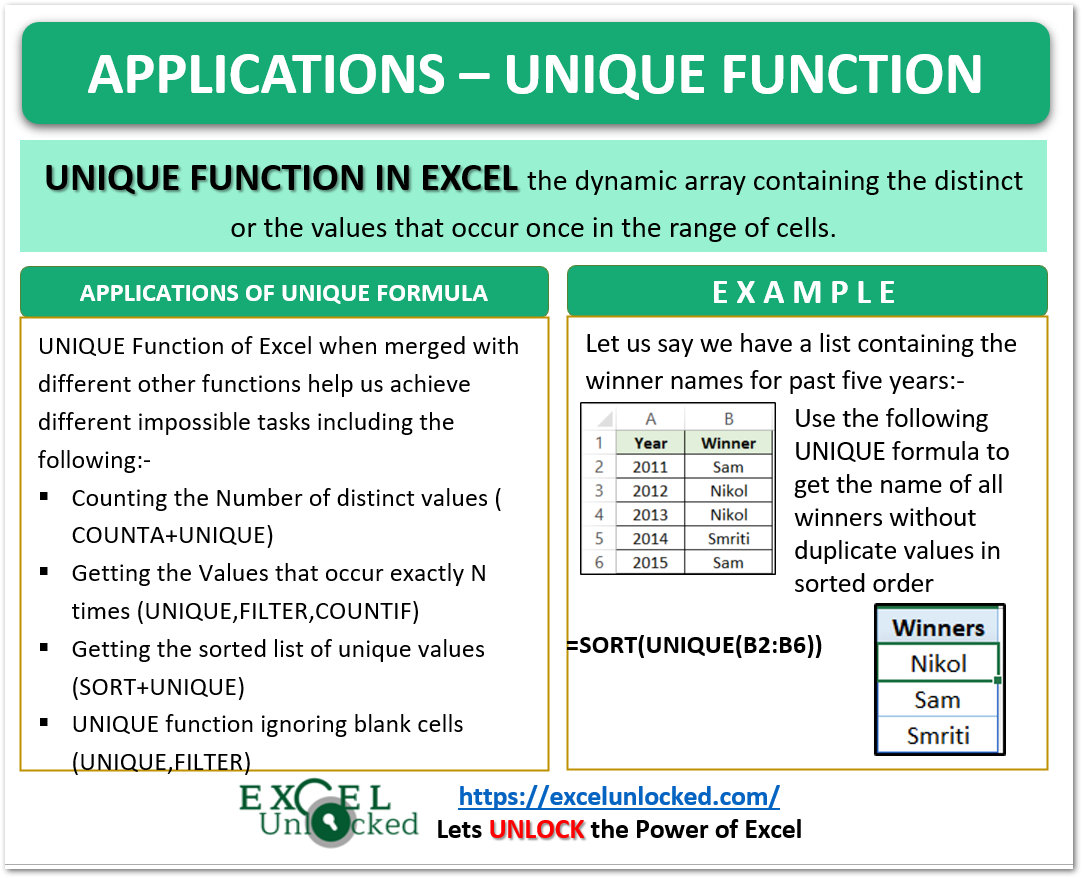
In the previous blog, we used the UNIQUE Function of Excel to understand the basic functionality of the UNIQUE Function. In this blog, we will merge the result of the UNIQUE Function with some other formulas to accomplish those tasks that would not be possible without the UNIQUE Function! So let’s get started learning the Applications of UNIQUE Function in Excel.
1st Application – Counting the number of Distinct Entries
Let us suppose that we have the order history of a restaurant serving different dishes as follows:-
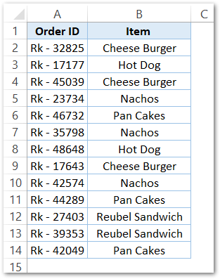
You can see that one item has been ordered multiple times, but we want to get the number of distance food items available in the restaurant from this list. Use the following formula:-
=COUNTA(UNIQUE(B2:B14))
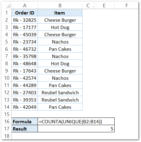
As a result, you will see that the formula has returned 5. So there are five items available in the restaurant. The items are Cheese Burger, Hot Dog, Nachos, Pan Cakes, and Reuben Sandwich.
We have used the COUNTA function with the results of the UNIQUE Function.
2nd Application- Getting the Values that occur Exactly N times
The UNIQUE function has the capability to return the distinct cells or the cells that occur exactly once. But what if we want to get the set of values that occur N times where N can be 1,2,3… or any natural number.
Let us suppose we have a list of winners of Basket Ball competition for the past 10 years as follows:-
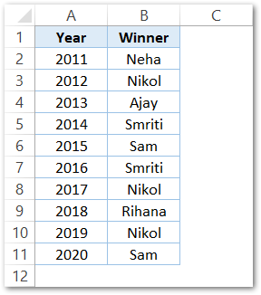
Let us suppose that we want the names of winners that won exactly two times (N=2)
We will use the following formula in cell D2:-
=UNIQUE(FILTER(B2:B11,COUNTIF(B2:B11,B2:B11)=2))
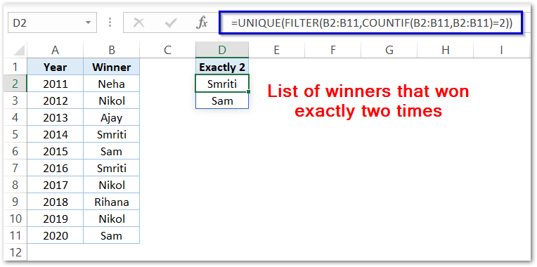
As a result, you can see that the formula has returned the name of two winners Smriti and Sam that won exactly two times in the past ten years.
The three functions UNIQUE, FILTER, and COUNTIF Function have been used together to give us this powerful formula. This is one of the most important applications of the UNIQUE Function in Excel.
Formula Explanation in Depth
Explanation – We have used the COUNTIF Function to get us the count of each winner in the range B2:B10:
Also Read: Applications – FILTER Function in Excel
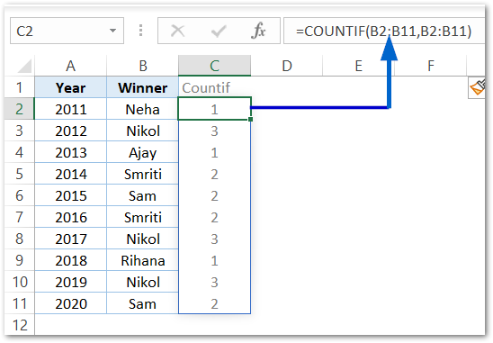
There after, we took the condition , that the count of each winner must be 2. This condition applies in our FILTER Function [FILTER(B2:B11,COUNTIF(B2:B11,B2:B11)=2)] that filters those rows.
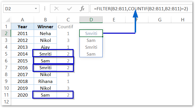
Lastly, we used the UNIQUE Function to get the names distinctly, since you can see we have two entries for each winner returned by the FILTER Function. The UNIQUE function returns the winner names returned by the FILTER Function.
Application 3 – Get the Sorted List of UNIQUE Values
Let us say we have the following list of winners as follows:-
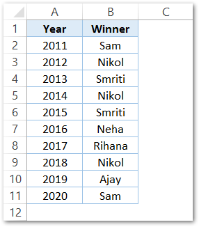
We want to get the list containing names of the winners but the duplicate values ( Sam in B2, B11 ) must be shown one time. The list must be sorted Alphabetically. We use the following formula.
=SORT(UNIQUE(B2:B11))
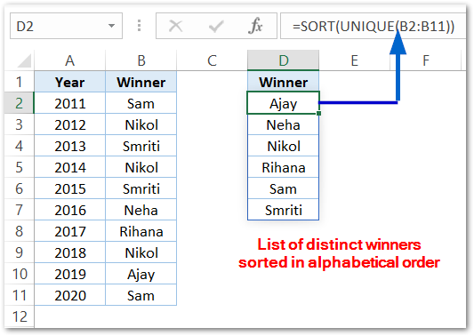
We have used the SORT function of excel, which sorted the list of distinct winners lists alphabetically.
Application 4 – Get Distinct Values by Ignoring Blanks
When we use the UNIQUE Function with a list containing blank cells, this is what happens:-
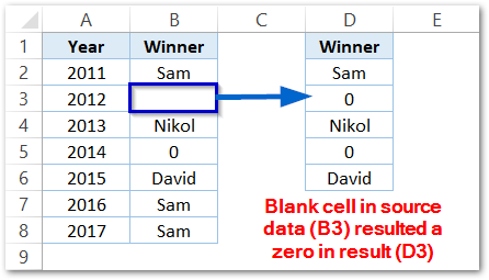
We can use the following formula to ignore those blank cells or cells containing zeros:-
=UNIQUE(FILTER(B2:B8,(B2:B8<>0)*(B2:B8<>"")))
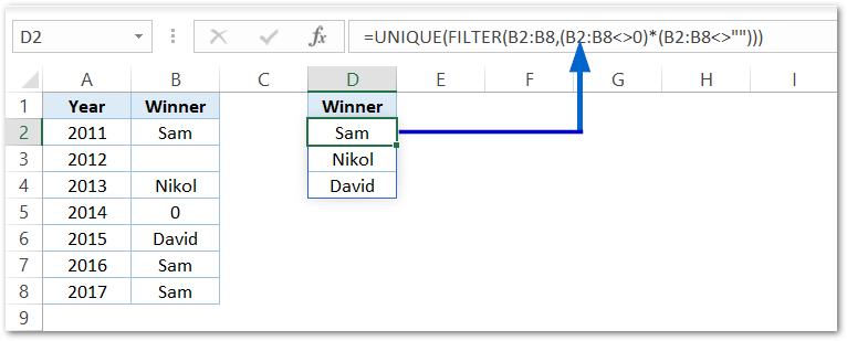
As a result, you can see that the formula has ignored the blanks (B3) and zeroes (B5).
Explanation – This is so because we have used the <> ( not equals ) operator in the condition specified by the FILTER Function. The FILTER function filters the cells in the range B2:B8 that is not equal to a 0 and is not a blank string (“”). The * implies AND Criteria.
This brings us to the end of blog.
Thank you for reading.
RELATED POSTS
- FILTER Function in Excel – Dynamic Filtered Range
- Applications – SUMPRODUCT Function in Excel
- Dynamic Array Formulas in Excel – Usage, Example, #SPILL
- How to Find Unique Values from Dataset In Excel
- ROWS Function in Excel – Get Number of Rows
- Excel COUNTIFS Function – Counting Cells with Specified Conditions

