Have you ever wondered how to find only unique values from a dataset in Excel? In this blog, we would unlock the technique to find and get the list of unique values from a dataset in Excel.
Example Data Containing Unique Values
Let us now understand this technique by taking a small example.
Below is the list of numbers that contains few values which are repeated multiple times and some values are unique i.e. they do not repeat.

Your need is to get the unique values from this list in a separate cell.
Find Unique Values from Dataset in Excel
Follow the below steps to find the unique values from the list of numbers.
Firstly, select the cell range containing the values. Hence, I have selected range A2:A15.
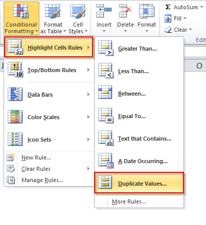
In the excel ribbon bar, select the tab “Home”. Under the “Style” group, click on the option “Conditional Formatting” as shown in the screenshot below:

From the drop-down list of options available, click on “Highlight Cell Rules” and then select the option “Duplicate Values”
Refer to the screenshot below:

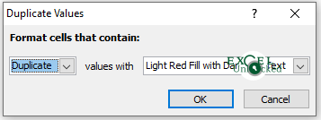
The “Duplicate Values” dialog box would appear on your screen:

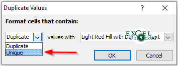
Now, click on the first downward facing arrow.
Two options would appear in the drop-down lists – ‘Duplicate’ and ‘Unique’.
Select the option “Unique” from the list of options in this drop-down list.

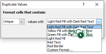
Another drop-down list is for how do you want the cells containing unique values to be formatted. You can select any option of your choice from the list of available options.

Accordingly, I have selected the first option “Light Red Fill with Dark Red Text”.
Now click on the “OK” button to apply the dialog box changes.
Finally, you would notice that the cell containing the unique value changes its color.
Refer to the screenshot below:

To get these values at some other location, just filter the highlighted cells and copy and paste them to the location of your choice.
This brings us to the end of this blog. Share your comments and view on this post in the comment section below.

