Do you know how to extract the values in multiple lines in the cell in Excel? In this blog, we would unlock the technique to extract the data in multiple lines. You would, in this blog, basically learn two ways. The first one is to extract the values in multiple lines into a single cell (using comma as separator) and the other is to extract the values in multiple lines into multiple cells (using text to column functionality).
Let me first make you understand, what is meant by ‘Values in Multiple Lines’.
By ‘Values in Multiple Lines’ we mean that there is a line break in the cell. You can insert the line break by using the Alt+Enter key on your keyboard. Below is one demonstration of the line break for your reference.

Now when you know what is a line break and how to apply a line break in a cell, let us begin with this tutorial.
As I mentioned earlier in this blog, we would learn two ways to extract the data in multiple lines in a cell. Let me first give you a brief about what are those two ways and what are we going to ultimately achieve.
Method 1
In the first method, we would extract the values and put those values in a single cell separated by a comma.
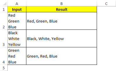
Method 2
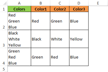
Another way, wherein, we would extract the values from multiple lines in a cell and put those in different cells horizontally like the way it is shown in the below image:
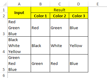
Let us now start with this technique and unlock the power of excel for you.
Sample Data
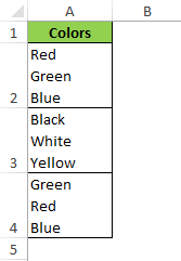
Before starting with this lesson, let us first make our sample data ready.
Enter the below sample data in an Excel worksheet.
Extract Values into Single Cell (With Comma Separator)
To extract the values into single cells (with commas as separator), we can either use the formula-based approach or use the ‘Find and Replace’ functionality. Let us first start with the formula-based approach.
Formula Based Approach
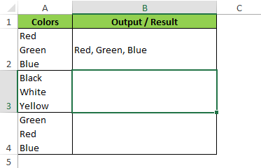
To extract the values in column A into a single cell (separated by comma), enter the following formula in cell B2:
=SUBSTITUTE(A2,CHAR(10),”, “)
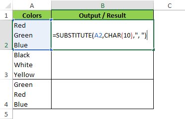
As soon as you press the ‘Enter’ key on your keyboard, you would notice that the excel extract the values in cell A2 and puts it into cell B2 (separated by commas).
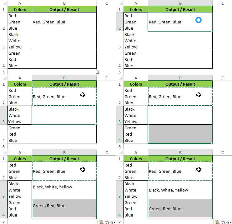
Copy cell B2 and paste it to the other cells in column B as demonstrated in the image below:
This brings us to the end of this method. Let us now learn the same using ‘Find and Replace’ functionality.
Using Find and Replace Functionality of Excel
Follow the below steps to achieve the result as shown above:
Extract Text in Multiple Lines Using “Find and Replace”
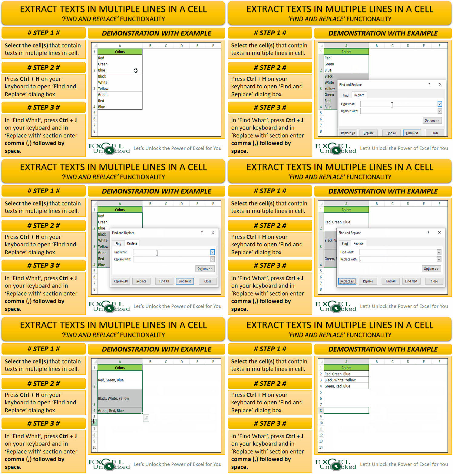
- Step 1
Select the cells that contain the values (In our case, I have selected cells A2:A4).
- Step 2
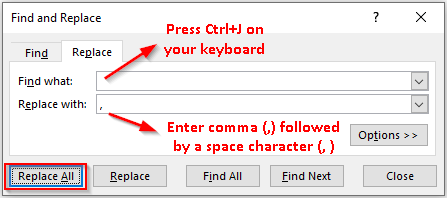
Press Ctrl+H on your keyboard to open the “Find and Replace” dialog box.
- Step 3
In the ‘Find What’ section, press Ctrl+J on your keyboard. You would notice that the ‘Find What’ section still remains blank (but that’s absolutely fine).
- Step 4
In the ‘Replace With’ section, enter ‘Comma’ (,) and then press ‘Space’ key on your keyboard.
- Step 5
Finally, click on the ‘Replace All’ button to activate it.
What did you notice? Surprised !!
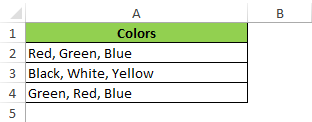
You can see that the texts which were earlier in multiple lines in a cell are now in a single line (separated by commas).
Extract Values into Multiple Cells (Using Text to Column Function)
Unlike the above method, this is not a formula-based approach. We would be using Excel ‘Text to Column’ functionality to achieve it.
Follow the below procedure to Extract values present in a single cell into multiple cells
Select the cells that contain values in multiple lines in a single cell (with line break).

In the ribbon bar, click on the tab “Data”. Now click on the button “Text to Column” under the “Data Tools” group.

To learn the Excel ‘Text to Column’ functionality in detail, visit and go through our previous blog on Using the Text to Column Functionality of Excel.
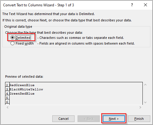
The “Convert Text To Column Wizard” dialog box wold open on your screen.
Select the radio button ‘Delimited’ and click on the “Next” button.
In the second step of this wizard, untick the ‘Tab’ checkbox and tick the ‘Other’ checkbox.
Now, comes the most important step of this technique.
Click on the input box besides the ‘Other’ checkbox and press Ctrl+J on your keyboard.
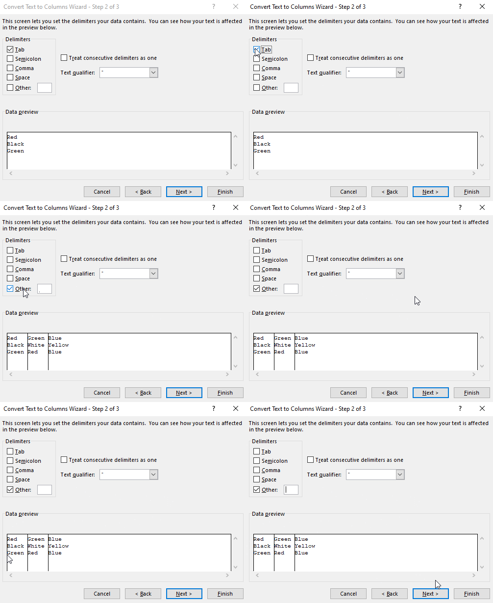
You would notice a change in the preview section of this dialog box. A vertical line divides all the colors.
Now, click on the ‘Next’ button to move to the next step of this wizard.
This is the third and last step of this wizard, where we shall select the destination cell. Click on the input box besides the ‘Destination’ and enter the destination cell reference (In our case cell B2) and then click on the “Finish” button to exit.
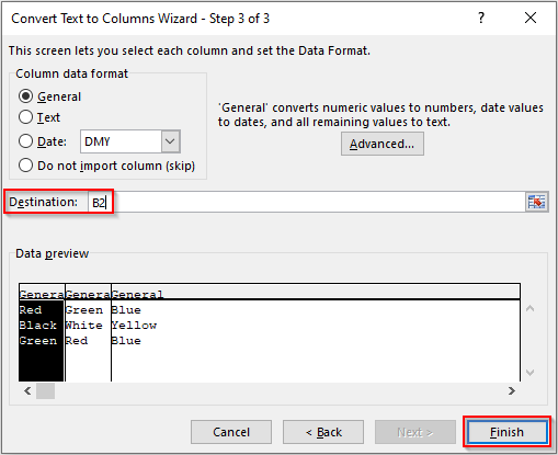
You would notice that the colors in multiple lines a single cell are now in different cells.
This brings us to the end of the blog.
