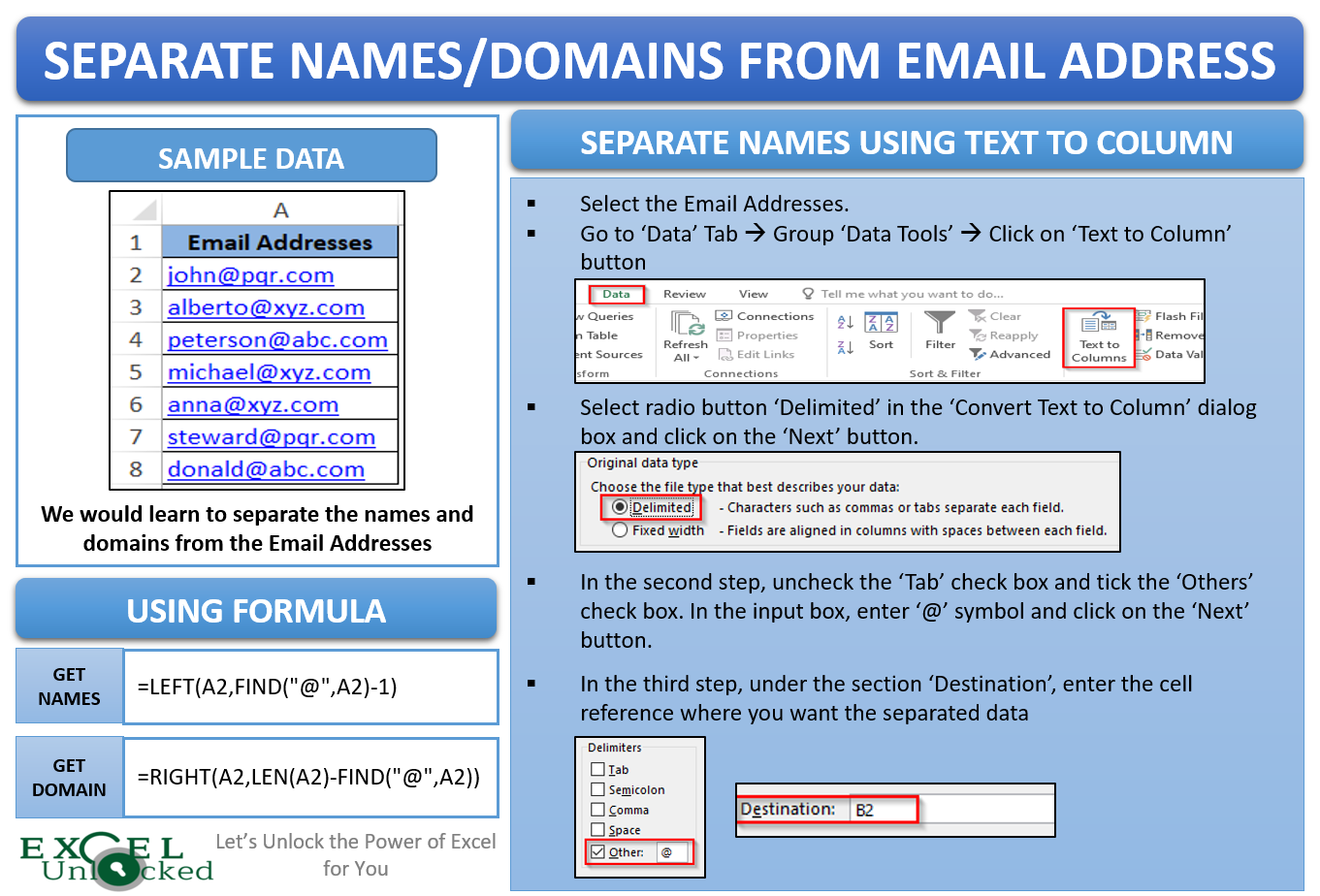
Many a time, you may have a list of email addresses in an Excel worksheet and you may wish to separate or get the name from those email address. Or you may even wish to get the domain name from the email addresses. There are multiple ways to do so. In this blog, we would unlock different ways using which we can get the name or domain from the email address in Excel.
So, let us first make our sample email addresses ready.
Sample Data
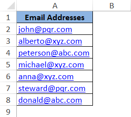
Below you can see the list of email addresses in column A in an Excel worksheet
As mentioned earlier, you can separate the names from the email addresses using different ways. We would here learn two of those methods.
The first one is a relatively easy method and does not require any formula. We would achieve it by using the Text to Column functionality of Excel.
The second method is a formula-based method. Here, we would use the formula to separate names and domains from the email addresses.
Let us now start with each of the methods one by one.
Get Name from Email Address – Using ‘Text to Column’
The ‘Text to Column’ functionality helps us to split the text into multiple cells by using a simple step by step wizard. To learn more about ‘Text to Column’ functionality of Excel, refer to our previous blog on ‘Using the Text To Column Functionality of Excel’
Follow the below step by step procedure.
Select the cell range (A2:A8).
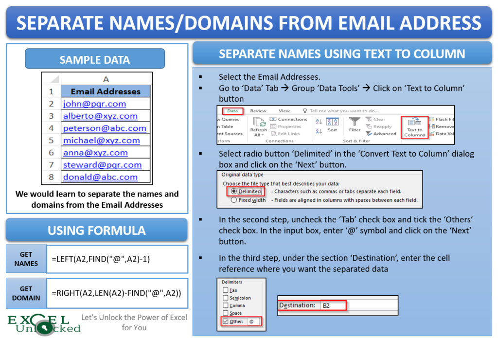
Now, click on the ‘Data’ tab. Under the group, ‘Data Tools’ click on the option ‘Text to Columns’.

The ‘Convert Text to Column Wizard’ dialog box would appear on your screen.
As we know that in our email addresses, the names and the domain names are separated by ‘at the rate’ symbol (@), hence it would be appropriate to use the ‘Delimited’ function of ‘Text to Column’ functionality of Excel.
Therefore, select the radio button ‘Delimited’.
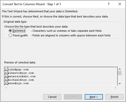
Now click on the ‘Next’ button.
As we know that the names and domains are separated by @ symbol, therefore, uncheck the checkbox ‘Tab’ and select the checkbox ‘Others’.
In the input box (besides the Others option), enter the separator @ symbol.
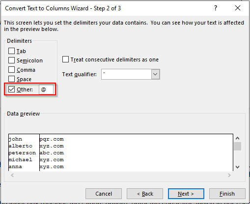
Now, let us move to the next and the final step of this wizard.
Click on the ‘Next’ button.
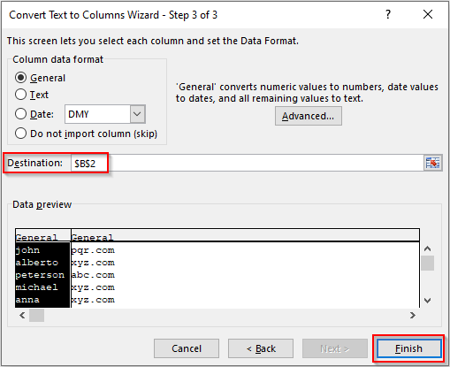
In the third and the last step of this wizard, we need to provide excel with the destination cell (where the delimited data will be placed).
Enter ‘$B$2’ in the destination section of this dialog box as shown in the screenshot below and then click on the ‘Finish’ button to exit this wizard.
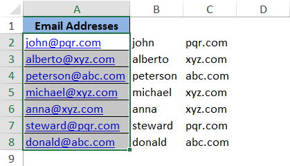
Finally, the excel separates the names and domain from the email addresses in columns B and C respectively.
Now, let us learn how to use the formula to separate names and domains from email addresses in Excel.
Get Name from Email Address – Using Formula
In the above method, we learned to separate the names and domain from the email addresses using a non-formula based approach.
In this method, we would do the same using a formula.
To get the names, enter the following formula in cell B2:
=LEFT(A2,FIND(“@”,A2)-1)
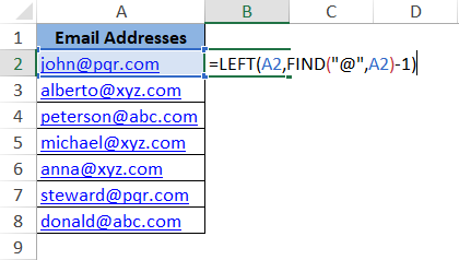
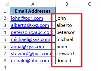
You would notice that the excel returns the name from the entire email address.
Now copy this cell B2 and paste it to the other cells in column B.
Resultantly, you would get the names extracted from the email addresses. Refer to the image below:
Explanation of Above Formula
We have used the LEFT formula of excel to get the names from the email address. The LEFT formula returns the string (up to the number of characters specified) starting from the left of the cell.
The first attribute of the LEFT formula is the reference of the cell which contains the text (in our case it is cell A2). The second attribute of the LEFT formula is the number of characters. By entering this attribute, we provide excel with the information that up to how many characters the excel should return the value. As the number of characters is different for each email address, therefore, we have given another formula FIND(“@”,A2)-1. This formula finds the position of “@” in the text in cell A2 and then reduce that value by 1.
Separate Domains from Email Addresses – Using Formula
Similarly, to extract the domains from the email addresses, enter the following formula in cell C2:
=RIGHT(A2,LEN(A2)-FIND(“@”,A2))

The excel returns the domains from the entire email address.
Now copy this cell C2 and paste it to the other cells in column C.
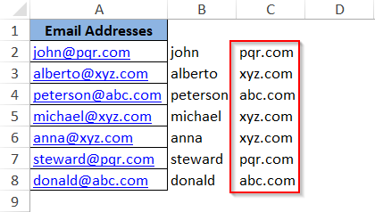
Explanation of This Formula :
We have used the RIGHT formula of excel to get the domain from the email address. The RIGHT formula returns the string (up to the number of characters specified) starting from the right of the cell.
The first attribute of the RIGHT formula is the reference of the cell which contains the text (in our case it is cell A2). The second attribute of the RIGHT formula is the number of characters. By entering this attribute, we provide excel with the information that up to how many characters the excel should return the value. As the number of characters is different for each email address, therefore, we have given a formula as the second attribute LEN(A2)-FIND(“@”,A2). This nested formula first finds the number of characters in the text in cell A2 and then reduces the position of “@” in cell A2.
This brings us to the end of this blog. Please, share your views and comments in the comment section at the end of this blog.

