The FIND Function in Excel is a useful function and is good to combine with other text functions of Excel. FIND Function has a variety of Applications. We will go from revising the fundamentals and then moving to advanced FIND formulas,
Here we go.
Revising the Fundamentals behind FIND Function
The FIND Function of Excel returns the position of one text string in another text string. The FIND Function can be used to tell if the substring is contained in a text string or not.
- A #VALUE! error is returned if within_text does not contain find_text.
- If you pass the value of start_num as 0 or a negative value, the FIND formula returns a #VALUE! error.
- The FIND function is case-sensitive. In other words, “T” and “t” would be considered as different characters.
- If the text string that we are looking for, occurs more than one time in the main string, then the function returns the position of the text string that occurs first from the left of the main string.
Required Inputs for FIND formula
=FIND(find_text,within_text,[start_num])
The following points contain the information about the FIND Function arguments
- find_text – This argument represents the substring that might be contained in the main text string.
- within_text – It is the text string in which we are looking for the substring.
- start_num (default – 1 ) – This is an optional argument. It is the position of the character from which we want to start our search of find_text in the within_text.
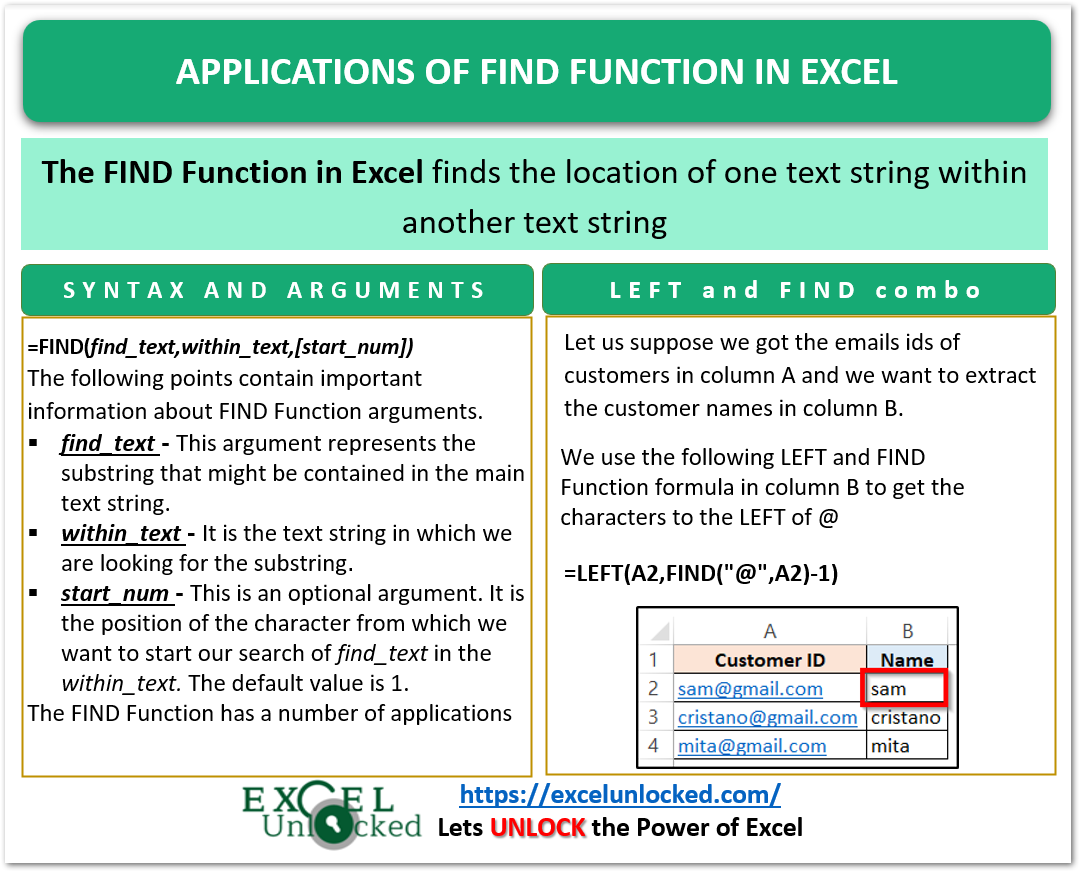
Applications of FIND Function in Excel
Until now, you must have been thinking of what do I have to do with the position of one text string within the other. This section of the blog is the answer to that! We are going to implement the Applications of FIND Function in Excel.
Application 1- Extract the Text String before a Specified Character
If there is any perfect combination of two functions that exist in Excel, then it is the LEFT and FIND function combination. LEFT Function extracts a specified number of characters from the left of a text string.
Let us say, below are the customer email IDs of a company.
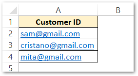
We want to extract the names of customers from their email IDs. Use the following Excel Formula.
=LEFT(A2,FIND("@",A2)-1)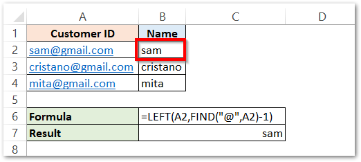
Consequently, the formula has returned the customer’s name as sam. We have copied the formula for the rest of the email ids.
Explanation – The FIND function in the formula returns the position of “@” (find_text) from the email id “[email protected]” (A2 is within_text). The position is 4. The number of characters including “@” turned out to be 4, which is “sam@”
But since we only want the customer name without the @ sign at the end, we need to subtract 1 from the FIND formula result to exclude the “@” from its position in the email id.
=LEFT(A2,4-1)
=LEFT(A2,3)
Now, the LEFT function will extract the 3 characters before “@” which is the name of the customer “same”
The same concept works for the remaining email ids. The FIND function returns the number of characters before “@”. The characters to the left of “@” will be extracted by the LEFT function.
This formula automatically locates @ using FIND Function and the LEFT function extracts the name from the left of @
Application 2 – Extract the Text String Followed by a Specified Character
In this example, we are going to combine three functions, RIGHT, LEN and FIND Function.
Suppose that we have got the following product code for different products.
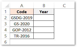
We want to extract the year from the product code, You can see that year occurs after a – symbol in each product code Therefore, we would extract it from the right of the product code. Use the following formula in cell B2.
=RIGHT(A2,LEN(A2)-FIND("-",A2))Copy the formula down the range A2:A5.
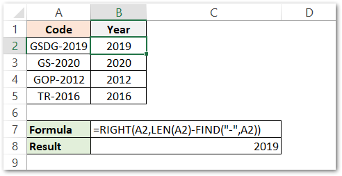
As a result, we got the product year in column B.
Explanation – The RIGHT function extracts LEN(A2)-FIND(“-“, A2) number of characters from the cell A2 containing the product code.
The length function returns the length ( 9 ) of the product code and the finds function returns the location of “-” ( 5 )in the product code,
LEN(A2)-FIND(“-“,A2)
The two outputs are subtracted.
9-5=4. 4 characters are extracted from the right of the product code.
Application 3 – Checking If one Text String Contains in Another
In this example, let us say we only want to know if the text string is contained in another text string or not.
The soul concept is, that the FIND function returns a #VALUE error if within_text does not contain the find_text. We got two examples here when we look for the location of find_text in within_text using the FIND Function and got the results.

ISNUMBER Function returns a FALSE if there is any other thing passed as input that is not a numerical value. We will use the following formula to get the required results.
=ISNUMBER(FIND(A2,B2))
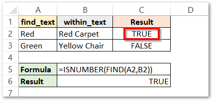
Therefore, the function returns a logical TRUE and FALSE in two cases.
Explanation – We have supplied the result of the FIND Function as the ISNUMBER functions’ argument. Whenever the FIND function locates the text string, it returns its numerical location. In this case, the ISNUMBER is inputted with a number and it returns TRUE.
On the other hand, if the FIND formula didn’t find the find_text in within_text, it returns a #VALUE! error. This error is not a numerical value, when it becomes the input of the ISNUMBER function, we get a FALSE as result.
The FIND formula has located text string “Red” in the “Red Carpet”. The FIND function returns 1.
=ISNUMBER(1)
This makes the result to be logically TRUE.
In the next row, the FIND function returned #VALUE! error because “Yellow Chair” does not contain “Green”.
=ISNUMBER(#VALUE!)
As a result, the formula returns a logical FALSE.
This brings us to the end of the Applications of FIND Function in Excel blog. Thank you for reading.
