The TRIMMEAN is another important statistical function in Excel. The TRIMMEAN Function is very easy to understand so let’s start learning the fundamentals of the formula.
When to Use TRIMMEAN Function in Excel?
The TRIMMEAN Function calculates the truncated mean for a data set containing numerical values. The Truncated mean is different from the average value.
The TRIMMEAN Function excludes a percentage of extreme values from the top and bottom of our data set. These extreme values are called outliers. An equal number of values are excluded from both the top and bottom of our data and the average of middle values is considered a Truncated Mean.
TRIMMEAN Function was introduced in Excel 2007 and can be implemented in later versions of Excel.
Syntax and Arguments
=TRIMMEAN(array,percent)
The following points contain information regarding the inputs required by TRIMMEAN Formula.
- array – This refers to the actual data set containing numerical values. We can supply a range, named range or direct numerical values in brackets.
- percent – Here we tell the function, the percentage of values that we don’t want to include from the top and bottom of our data in the resultant mean.
What is the 10%, 20%, or 15 % Trim Mean in Excel?
Let us suppose we have got 20 numerical values in the data set. When we say we want a 10% Trimmed Mean of this data, then 10% of the 20 numerical values – 2 excluded values in total. One from the top and the other from the bottom would be excluded while calculating the average.
Similarly, a 20% Trim mean would exclude 20% of the 20 numerical values – 4 values to be excluded in total. This means that 2 values from the top and two from the bottom would not be considered while calculating central tendency.
An important point to mark is that the TRIMMEAN formula excluded an equal number of values from both the top and bottom of the data set. Therefore, the total number of excluded values is always in a multiple of 2.
Example – When we want to calculate a 15% Trim Mean for a data set having 20 values – 3 values to exclude in total. Since 3 is not a multiple of 2, a value lower than three would be the total number of excluded values. Therefore, the 2 values in total, one from the upper range and one from the lower range would be discarded.
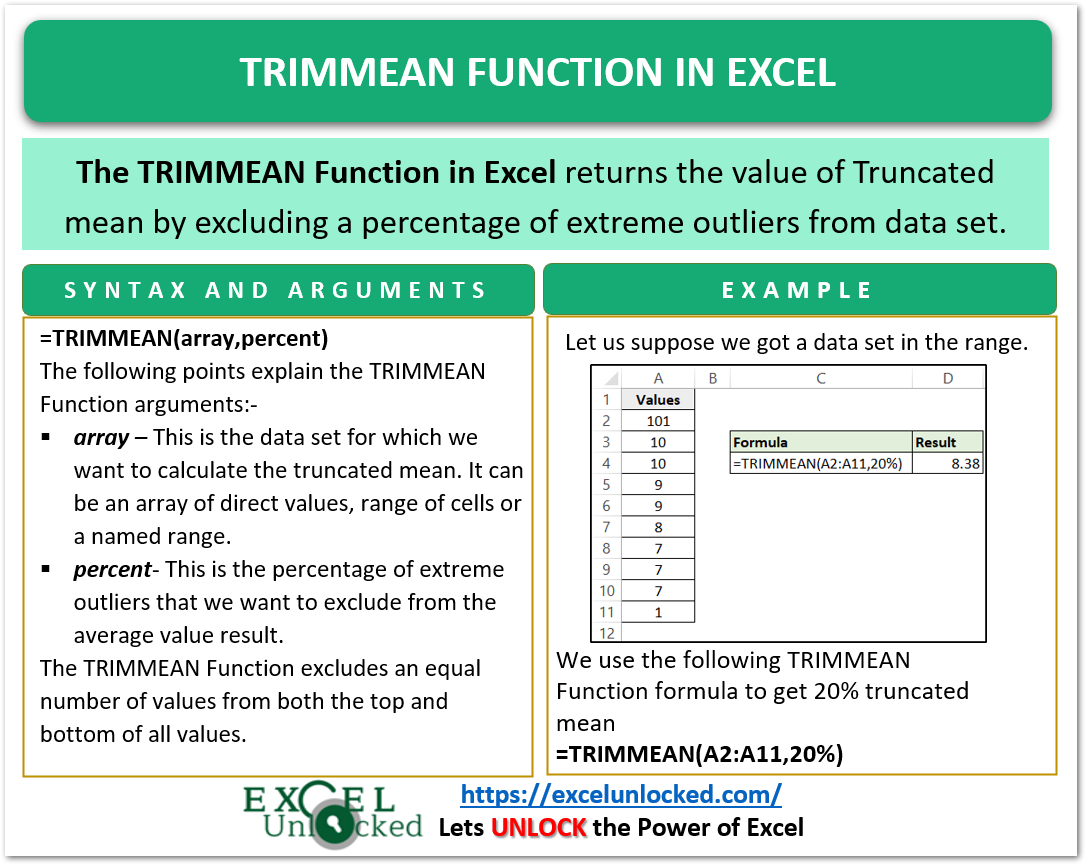
Examples to Learn TRIMMEAN Formula
In this section, we are going to implement the TRIMMEAN Function as follows.
Example 1 – Basic Example for TRIMMEAN Function
let us suppose we have got the following data set containing 10 numerical values in the range A2:A11.
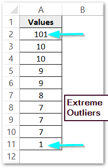
You can see that most of the values lie between 10 and 7 while there is one value of 101 on top and 1 at the bottom. These values are Extreme outliers as they are extremely different from other values.
This is exactly when we need the TRIMMEAN function for these outliers to not affect the average of this data.
Use the following TRIMMEAN formula to calculate the 20% Truncated Mean for this data.
=TRIMMEAN(A2:A11,20%)
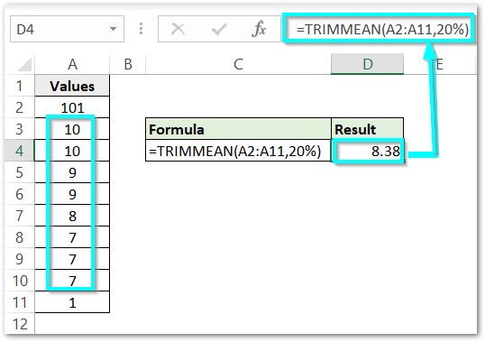
As a result, we get the average value as 8.38
Explanation – the numerical data set is contained in the array of cells A2:A11 which becomes the array input of the TRIMMEAN formula. The percent input is 20% as we wanted to get a 20% Truncated mean.
The function excludes the 20% of 10 values – 2 values would be excluded. One from the top and one from the bottom which is easily noticeable in the example, 101 and 1 respectively ( because we have sorted data ). The average of the remaining values becomes the TRIMMEAN formula result.
Example 2 – 25% TRIMMEAN for Data
Here, we got the monthly sales of a company past year as follows.
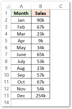
Use the following TRIMMEAN formula of Excel to get a 25% Truncated Mean.
=TRIMMEAN(B2:B13,25%)
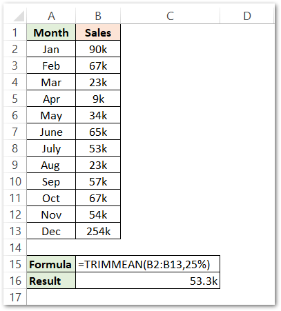
As a result, we got the average sales as 53.3k
Explanation – We have supplied the range B2:B13 as the array input of the TRIMMEAN formula that contains monthly sales. The percent argument is 25%,
The 25% of 12 values is 3. Since 3 is not a multiple of 2, a value less than 3 would be considered for outliers. 2 values in total would be excluded from the average sales.
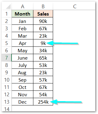
The sales of April and Dec would be excluded from the average of sales as they are the lower and upper outliers. Therefore, the average of sales for 10 months (excluding Apr and Dec ) becomes the formula result.
This brings us to an end.
Thank you for reading.
RELATED POSTS
- AVERAGEA Function in Excel – Finding Average Value From All
- PERCENTILE.INC Function in Excel – Inclusive Function
- AVERAGEIF Function In Excel – Finding Average With Condition
- AVERAGE Function in Excel – Finding Mean or Average Value in Excel
- Excel AVERAGEIFS Function – Multiple Criteria Average
- ROUND Function in Excel – Normal Rounding in Excel
