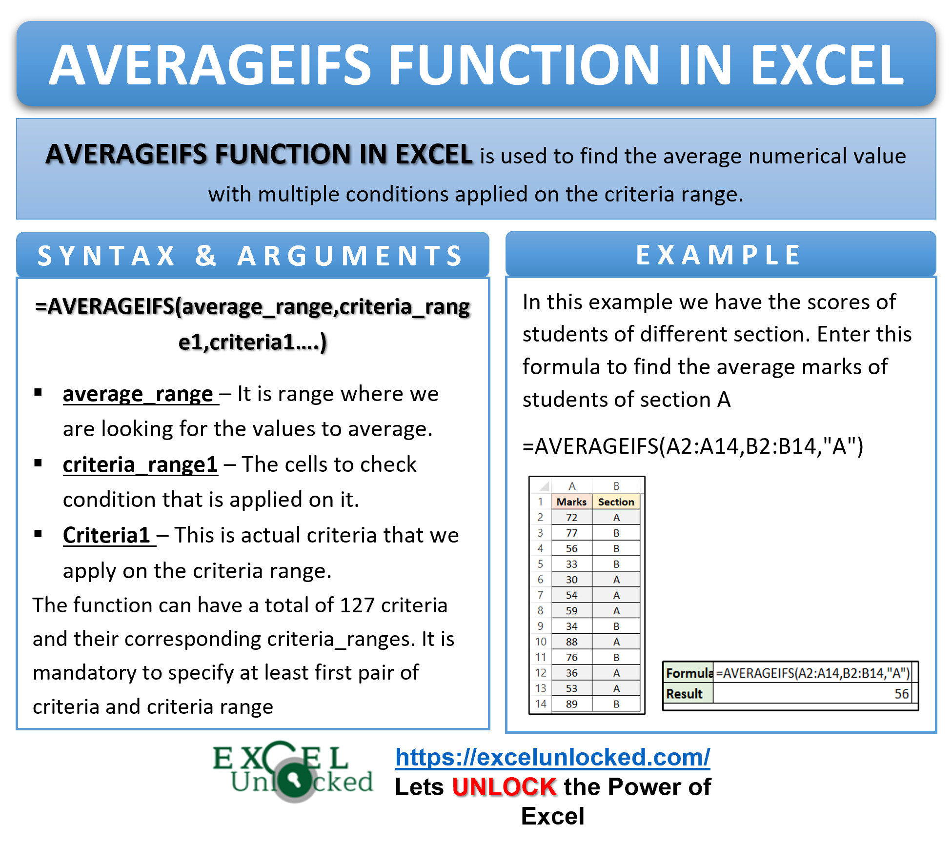
In our recent blog, we learned how to use the AVERAGEIF function to find the average by applying one condition. In a similar manner, the AVERAGEIFS function in Excel also helps in finding the average in excel, with a slight difference. Unlike the AVERAGEIF function, you can apply multiple check conditions to find the average.
This tutorial explains the AVERAGEIFS formula in excel, its usage, syntax, arguments, and examples.
Let us begin 😎
When To Use Excel AVERAGEIFS Function
The expression AVERAGEIFS represents “Average value with multiple IF”. The excel AVERAGEIFS function is used to find the average of values in excel where more than one (multiple) conditions satisfy.
This function can be used to know the average balance in the inactive bank accounts with an updated KYC. Similarly, the function can also find the mean score of marks that were 90 plus marks from section A.
Syntax and Arguments
=AVERAGEIFS(average_range,criteria_range1,criteria1,…)
- average_range – In this argument, specify the range to look for the average value.
- criteria_range1 – In this argument, specify the range on which you want to apply the criteria.
- criteria1 – In this argument, specify the actual condition to apply on the criteria_range1.
The function has a maximum of 127 pairs of criteria and criteria_range.
Must To Know Points – AVERAGEIFS Formula in Excel
Keep these points in mind before actually using the AVERAGEIFS formula.
- The average_range and criteria_range should have the same size.
- The function ignores logical values (TRUE and FALSE) and text strings when present in average_range.
- When using logical operator (<, >, <>, =) in the criteria :-
- Enclose the text strings and dates within double quotes (“”). For example, “Excelunlocked” or “>10/10/2021”.
- Use ampersand symbol (&) between the logical operator and the cell reference or a number, or formula. For example, “>”&15 or “>”&A15.
- While using wildcard characters with the AVERAGEIFS function criteria1
- Put the wildcard character and the text string within a double quote. For example, “*Excelunlocked”
- Concatenate wildcard character and the cell reference using ampersand symbol. For example, “*”&A2.
- The function will return a #DIV/0! error if no record satisfies the criteria in the criteria_range.
- The function will return a #VALUE! error if the size of average_range and criteria_range is not same.
- For multiple criteria, the function will find the average value of the records that satisfy ALL the conditions.
Examples to Understand AVERAGEIFS Function in Excel
Let us now check out some examples to learn the actual usage of the AVERAGEIFS function in Excel.
Ex. 1 – Passing Mandatory Argument to AVERAGEIFS Formula
The below example image shows the marks obtained by students involved indifferent Co-curricular activities.
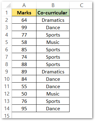
Suppose, we want to know the average marks of students involved in ‘Sports’ co-currricular activity.
To get the desired output, use the following AVERAGEIFS formula:
=AVERAGEIFS(A2:A14,B2:B14,"Sports")
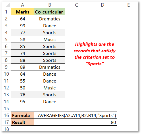
As a result, the function returns 80.
Explanation – In the above example, the average_range is A2:A14 containing marks of students from all the fields. The criteria “Sports” applies to the criteria_range B2:B14. The cells that contain the text string “Sports” within the criteria_range B2:B14 are B4, B6, B7, B8, B13. Consequently, the function calculates the average of corresponding records from the average_range as 80.
Ex. 2 – Using Multiple Criteria In the Excel AVERAGEIFS Function
Let us suppose, there is an order dispatching company. The below image contains dispatch details to various areas.
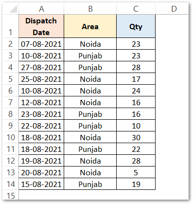
Now, suppose we wish to find the average quantity of products to Noida, not sent till today.
To get the required output, we need to use the TODAY formula in excel along with the AVERAGEIFS formula:
=AVERAGEIFS(C2:C14,B2:B14,"Noida",A2:A14,">"&TODAY())
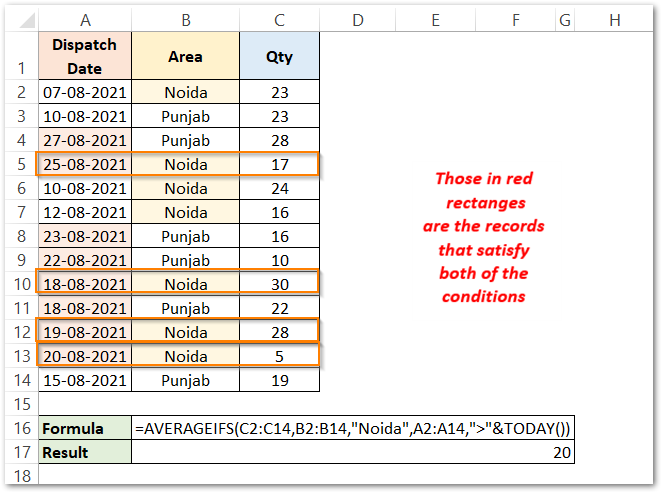
As a result, the above formula has returned 20.
Explanation – In the above example, the average range is C2:C14. The criteria “Noida” applies to the first criteria_range B2:B14. The cells that satisfy the first condition are highlighted in orange. The second criteria “>”&TODAY() applied on the criteria_range2 A2:A14. The cells that have dates greater than today’s date (17-08-2021) are in red. The function looks for the records that satisfy both of these conditions simultaneously i.e. cells C5, C10, C12, C13. Finally, the AVERAGEIFS function finds and returns the average of the values in these cells.
Ex.3 – Using Wild Card Characters with Excel AVERAGEIFS Formula
Wild card characters in Excel are used when we do not know the exact match for what we are looking for. There are mainly two wildcard characters in excel–
- ? (question mark) for one character match
- * (asterisk) for a sequence of character matches
The below image shows information about monthly sales of different bakery items.
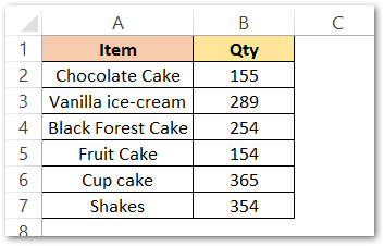
Now, let’s find the average sales for the cakes irrespective of the type. To get the desired output, use the following formula:
=AVERAGEIFS(B2:B7,A2:A7,"*"&D5)
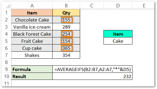
As a result, the formula has returns 232.
Explanation – The average_range is B2:B7 (where we are looking for the average result). The criteria apply to the range A2:A7. The criterion is “*”&D5. The cells that contain the sequence of characters (“*”) before the text string “Cake” (&D5) in the range B2:B7 will satisfy this condition. The highlighted records satisfy this condition and the corresponding values in the average range (B2, B4, B5, B6) gives the formula result as 232.
Thank you for reading 🙂
RELATED POSTS
- AVERAGEA Function in Excel – Finding Average Value From All
- RANK.AVG Function in Excel – Usage, Error Handeling
- TRIMMEAN Function in Excel – Truncated Mean
- HARMEAN Function in Excel – Get Harmonic Mean
- MEDIAN Function in Excel – A Statistical Parameter
- AVEDEV Function in Excel – Definition and Examples

